DIVULGACIÓN de PROYECTOS I+D
Laboratorio Multidisciplinar de Ciencias Básicas
UTN Rosario
INTERACTIVO
Universidad Tecnológica Nacional - República Argentina
www.utn.edu.ar
Esta obra está bajo licencia Creative Commons 4.0 internacional: Reconocimiento-No Comercial-Compartir Igual. Todos los objetos interactivos y los contenidos de esta obra están protegidos por la Ley de Propiedad Intelectual.


DIVULGACIÓN de PROYECTOS I+D
Directora:
Laboratorio Multidisciplinar de Ciencias Básicas
Mg. Alicia María Tinnirello
Co-director:
Eduardo Alberto Gago
Integrantes:
Lucas D’Alessandro
Mónica Dádamo
Matías Romero
Paola Szekieta
Mariano Valentini
Rosario, 2018.
Divulgación de Proyectos I+D
Laboratorio Multidisciplinar de Ciencias Básicas - UTN Rosario
Interactivo
Alicia María Tinnirello, Eduardo Alberto Gago,Lucas D’Alessandro, Mónica Dádamo, Matías Romero, Paola Szekieta, Mariano Valentini
Librería turn.js: Emmanuel García
Diseño y programación del libro: Valeria Iliana Bertossi
Índice
Integration techniques in mathematical application projects for mechanical
engineering.11
Project learning environments in nechanical engineering education.31
Design, simulation and analysis of a fluid slow system through multiphysics
platform.85
Métodos de variable compleja en el estudio de la dinámica del flujo de calor.131
Análisis dinámico para la modelización de sistemas con funciones complejas. 183
5
Design and simulation of mechanical equipment by design tools and
multiphysics platforms. 211
Systems analysis and modelling techniques in physical domains.237
6
Diagnosis of rotor failures current power induction motors by spectral analysis
methods.299
Educational technology intervention for the develpment of advanced
calculus applications.333
Virtual instruments integrating mathematical modeling for engineering
education.359
Integrating mathematics technology with mechanical engineering
curriculum.391
Introducing discrete dynamic systems in algebra teaching process.423
Computational methods: their advantages on teaching complex fluid flow
systems.487
7
Modelización y Simulación
de Sistemas:
Matemática Computacional
y Tecnologías para la
Educación Multidisciplinar
en Ingeniería
Homologado por la Secretaría de Ciencia y Tecnología bajo la identificación Nº 25M/066
Fecha de inicio: 01/01/2013
Fecha de finalización: 31/12/2016
INTED 2012
INTEGRATION TECHNIQUES IN MATHEMATICAL APPLICATION PROJECTS FOR MECHANICAL ENGINEERING

Descargar pdf
Tinnirello Alicia María, Dádamo Mónica Beatriz, Gago Eduardo Alberto
Laboratorio Multidisciplinar de Ciencias Básicas
Universidad Tecnológica Nacional, Facultad Regional Rosario (ARGENTINA)
Abstract. In this article, the authors present the development of mathematical concepts in mechanical engineering, where a new methodology for computational-oriented mathematics education is performed. Finding new opportunities of applying new technologies in teaching and learning mathematics in the engineering community are increasing. Computational-oriented mathematics education in virtual learning environments has led to new possibilities for engineering work, in which complex mathematical problem solving with computer visualization and simulation plays a central role, and its developments incorporate numerical analysis and simulations. The study of dynamical
11
INTED 2012
system
stability is presented in a systemic way by using simple and compacted techniques, showing the
connection among different solving methods.
Linear time invariant dynamical systems are gradually developed to study the model that represents
the early feedback stage in simple description of physical phenomena. This approach facilitates
software engineering professionals when designing systems with controllers, where the feedback is
considered a main feature.
Our goal in this study of dynamical systems will be accomplished by using the linearity property
transfer function and feedback mechanisms as basement of their analysis and synthesis.
The integration of computer-oriented mathematics is very important for the educational process in
engineering as well as for improving their qualifications, in the sense that are considered real systems
and structures which solve real problems.
Keywords: feedback, modelling, transfer function, dynamical systems.
12
INTED 2012
1 INTRODUCTION
In the introduction to physical systems modelling and control systems design, information technologies
converge with advanced elements of mathematical calculation. Systemic and analytical paradigms,
from incompatible philosophical roots, overlap; giving rise to a pedagogical and didactic problematic.
Feedback, is treated here in relation with mathematics associated with the study of linear timeinvariant
systems (LTIS), being the primary focus of the proposed analysis. The feedback, as suitable
concept of modelling systems, has been incorporated to current science and technology after the
Second War World. [1] [2].
From multidisciplinary, cybernetic and systemic origin, feedback resists its incorporation to the
analytical body of classic physics [3] [4]. The Authors, engineering professors, consider introducing in
the early stage of the engineering curriculum the concept of feedback, in order to display the
compatibility between the treatment of systems by traditional ways, by means of differential equations,
and the one obtained through computational programs oriented to complex and
13
INTED 2012
control systems that use block diagrams and feedback arrows.
2 OBJECTIVE
The objective of this work is to link the analytical vision, present in classic physics, with the systemic
approach, key component of professional software’s for modelling and simulation, considering in detail
the following goals:
• Perform training on professional tools management.
• Link engineering work with basic science.
• Contrast systemic paradigms with analytical ones.
3 PRELIMINARY CONCEPTS
In order to build a meaningful learning, basic knowledge of Laplace transform and its application to
solve systems using differential equations are needed as an introduction of Block Algebra, as well as
knowledge about programming in graphic languages (Simulink, LabView, Xcos). In addition,
knowledge on transform function management, Fourier analysis and time-series frequency domain is
required.
14
INTED 2012
These concepts will give to the student an optimal view of the current state on scientific-technological development linked to LTIS of continue data, with the exception of recent systemic studies that exceed the objectives of the advanced basic training [5].
4 BASEMENT
On the study of systems and simple phenomena, it can be considered that an efficient handling of the
object under study is linked directly with the understanding of the topic. In complex systems, the
relationship between operational expertise and explaining and justifying areas, is potentially more
diffuse [6]. An example of the above is seen on the study of the LTIS, in which through its calculation,
it is jointly introduced with the learning, the Laplace transform, the Fourier transform, the transfer
matrix, the convolution theorem, etc.
One unexpected result of this combination of elements of LTIS would be to consider the respective
transfer function (TF) as "obtained through Laplace transform, when the entry is a unit impulse"
If focus is given on the inherent properties of linear
15
INTED 2012
systems, it is highlighted that the FT is
characterized by the linearity of the differential operator that describes the model, that constant
coefficients describe a time-invariant system and that we select the "side" that corresponds to the
system, making it independent of the input function.
With a LTIS is possible to link solutions obtained -from an analytical approach- by means of differential
equations with those obtained -from a systemic approach- with simulation systems by means of block
diagrams and feedback loops, and not as disjointed techniques among themselves.
This alternative way to obtain solutions for a differential equation is motivated by:
- Current control systems (as PID type), widely spread in industries where feedback is used in an
intrinsic form.
- The fact that, as the system become more complex, is greater the incidence of a computational
component over mathematics, as well as informatics moving towards the paradigm of object-oriented
programming, which can be objectively associated to blocks and algebra of blocks.
- The concept of feedback has recently being added to the field of science and technology; born in
World War II and with an
16
INTED 2012
interdisciplinary origin make difficult its incorporation into the basic
educational curriculum, which has centuries-old roots.
- Cybernetic and systemic "feedback", though it complements the engineering analytical vision,
refuses to be pigeonholed in the reductionism of the positive Sciences.
5 DEVELOPMENT OF METHODOLOGICAL APPROACH
A mass-spring damper system of mass one, with friction coefficient  and constant elastic
spring
and constant elastic
spring  is considered. It is assumed that both are linear and invariant in time and space, and
the system responds to an external force.
is considered. It is assumed that both are linear and invariant in time and space, and
the system responds to an external force.
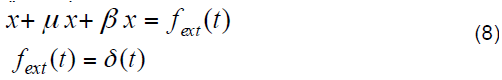
Analytical treatment based on Newton's laws or Lagrangian formalism leads to differential equation

If we assume a graphical interface proposal of the programs oriented to design control systems, guided by the program rules, the following figure summarizes, in a schematic way, how the same system is “thought”.
17
INTED 2012
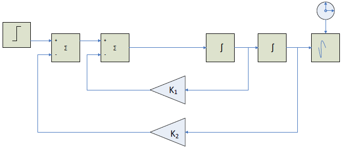
Fig.1 Model with feedback
In this instance, it is to remark that the traditional teaching methodology efficiently prepares to the intellectual treatment, synthesized in the equation (1); however, there is no enough emphasis on the formation of a mental archetype that allow the design of the Fig.1.
In Fig.1 we focus on the subsystem, which has an integrator block and a feedback, noted as G1. After treatment with block diagram algebra, the diagram complexity is reduced (Fig.2).
18
INTED 2012
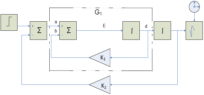
Fig.2 Block integrator selection and feedback
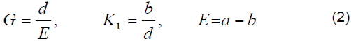
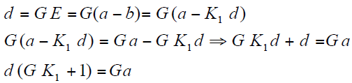
so
19
INTED 2012
then
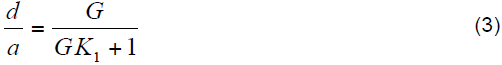
In order to synthesize the block as a whole, and considering 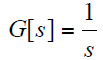 and
and  , where
  is the coefficient of dynamic friction. By means of a simple algebraic manipulation, is obtained:
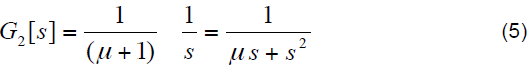
Calling G1 to G, to obtain G2 while the blocks in series are synthesized by multiplying their transfer functions (Fig. 3).
20
INTED 2012
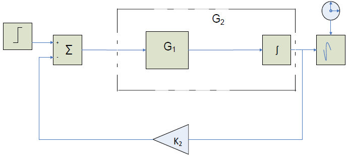
Fig.3 Second synthesis: series blocks
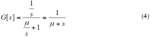
Fig. 4 shows the compacted second synthesis, which suggests a similar elaboration to the first one, changing the transfer function  by
by  and
and  by
by  , with
21
INTED 2012
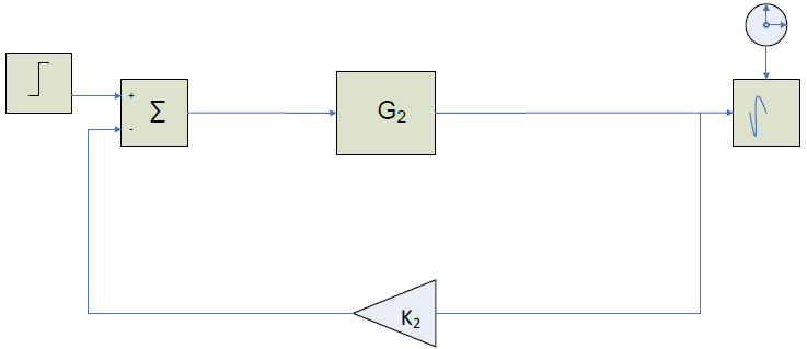
Fig.4 Simple feedback
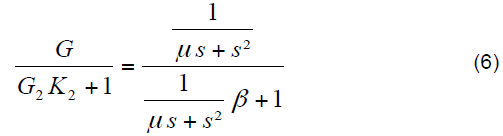
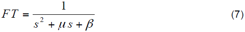
Applying elementary algebra rules in equation (6), can be obtained:
22
INTED 2012
This is equivalent to the transfer function obtained through modelling by means of ordinary differential equations. A mass-spring damper system as:
5.1 Analytical paradigm: a mass-spring damper system
Systems modelling, in the engineering basic training, are accessed by means of differential equations in accordance to the classic physic analytical view.
It is possible to use a wide variety of software (Matlab, Mathematica, Máxima, Scilab, Octave) for its resolution.
Fig.5 shows an example, where Mathematica software is used to solve differential equation stated on equation (8).
23
INTED 2012

Fig.5 Mass-spring damper system modelling by Mathematica
5.2 Systemic paradigm: mass-spring damper system
Professional environment for physical or industrial systems simulation (Simulink, Lab-View, Xcos) use a graphical mode as an interface with the user, characterized by block diagrams and
24
INTED 2012
their interaction, adding feedback loops. The latter has acquired special relevance as it is an essential part in any control system.
Using LabView software, simple and practically intuitively a graphic structure that model the system is developed, obtaining the answer to a particular entry, as shown in the Fig.6 and Fig.7.
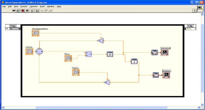
Fig.6 Mass-spring damper system modelling by LabView software
25
INTED 2012
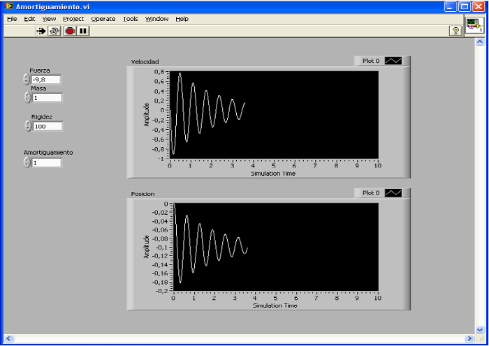
Fig.7 Answers to systemic model
6 CONCLUSION
To develop the present paper, though there are abundant
26
INTED 2012
pedagogic and didactic publications that use this concept in their essence, bibliography that explore the concept of the feedback from a conceptual point of view could not be found. [7] [8] [9].
During engineering degree education, feedback is treated in a technical way, generally associated with programs that implement it to treat of complex systems, with little or no mention of the systemic approach.
In this paper, the concept of feedback is shown efficient and compatible to manage Newtonian mechanic, and independent of the analytical paradigm. Even though, its way of relating shows a breakage with the traditional severity of the analytic approach, it is consistent with the paradigm of complexity, where analogical reasoning, coupled with its verifiable effectiveness, is considered valid.
In a simple way, an early mention of the systemic approach is done, an approach for which there is currently little academic treatment and is intensively used in professional engineering life.
In the university education, the LTIS, objects on which the feedback concept is applied with significant success, have a
27
INTED 2012
strong analytical basement and no systemic approach; they are taught associated with matrix or transform techniques, where mathematical elements from transformed functions are combined with the mathematics from the LTIS and its phase space. This confluence facilitates algorithm calculation but difficult conceptual and significant learning.
On the other hand, the use of transform functions, especially Fourier, is the traditional way to connect the domains of time and frequencies. Therefore when planning, designing and implementing curriculum strategies, it is necessary to avoid an "indoctrination", in a particular way to operate the LTIS and train the student to carefully select between the multiple mathematics and computing tools available to treat SLI, in particular to those that make use of blocks and feedback loops, linking these latter with basic curricular contents.
28
INTED 2012
REFERENCES
1. Rosnay J(1993). El macroscopio, hacia una visión global. Madrid: Editorial AC, 1993. Ch.2.
2. Pagels HR(1989). The dreams of reason, the computer and the rise of the sciences of complexity. New York: Bantam Books.
3. Arnoletto EJ(2007). Curso de Teoría Política. Available on http://www.eumed.net/libros/2007b/300/52.htm (Consulted 12/03/2011)
4. Shannon Claude E, Weaver W(1963). The Mathematical Theory of Communication (5th Ed). Chicago: University of Illinois Press.
5. Liu S, Lin Y(2010). Grey Systems. Theory and Application. Berlin: Springer-Verlag
6. Lilienfeld R(1984). Teoría de Sistemas. México DF: Trillas Ed.
7. Maldonado R, Eduardo C(2009). Sobre la retroalimentación o el feedback en la educación superior on line. Available on
29
INTED 2012
http://redalyc.uaemex.mx/src/inicio/ArtPdfRed.jsp?iCve=194215516009 (Consulted 11/30/2011)
8. Villardón Gallego L(2006). Evaluación del aprendizaje para promover el desarrollo de competencias. Educatio siglo XXI, 24: 57-76. Available on http://revistas.um.es/index.php/educatio/article/viewFile/153/136 (Consulted 12/03/2011)
9. Lorrie A. Shepard(2005). Formative assessment: Caveat emptor. Available on http://www.cpre.org/ccii/images/stories/ccii_pdfs/shepard
%20formative%20assessment%20caveat%20emptor.pdf (Consulted 12/04/2011)
30
ICERI 2012
PROJECT LEARNING ENVIRONMENTS IN MECHANICAL ENGINEERING EDUCATION Descargar pdf
Tinnirello Alicia María, Gago Eduardo Alberto, Dádamo Mónica Beatriz
Universidad Tecnológica Nacional (ARGENTINA)
atinnirello@frro.utn.edu.ar, egago@frro.utn.edu.ar, mbdadamo@gmail.com.ar
Abstract. Learning and training mathematical concepts and algorithms in engineering education require solve problems in projects as well as to communicate and present mathematical content. Every system can be described by a mathematical model, and the models can be applied in practice because the computers allow us to solve symbolically and also numerically from different design and performance. The technological advance demand changes in the curricula and in the way of teaching in higher education, where a new methodology for computationally oriented mathematics education is performed.
New opportunities by using new technologies in teaching and learning mathematics in engineering community is becoming increasingly. Then computational oriented mathematics
31
ICERI 2012
education in virtuallearning environments has led to new possibilities for engineering work in which mathematically complex problems solved in the computer by visualization and simulation play a central role.
To incorporate the opportunities offered by computer systems in increasing development and availability is necessary to design appropriate strategies. Mathematical software developments that have experienced and affinity with the students to engage with technology, require math teachers make the effort to transform the teaching-learning process in a process of learning by doing, in simulation learning environments.
The authors present in this proposal an innovative interdisciplinary design developed for learning advance calculus at third level course of Mechanical Engineering; understood technology as a tool that set ways of thinking and allow exploring modes of symbolic mental representation, constructed as a product of cognitive internalization skills from communication technology results, and becoming a tool of thought. Learning strategies are established based on different projects without neglecting the theoretical foundation, with a multidisciplinary approach.
32
ICERI 2012
The learning process is developed at a laboratory session, impossible to reach without technology, the way of teaching basic sciences, taking into account the importance of using computer networking, connecting computers that support electronic lab notebooks, data acquisition and analysis, graphics and report preparation are the central issues presented in this work.
Keywords: Modelling, Simulation, Computational Mathematics, Virtual Laboratories.
1 INTRODUCTION
New opportunities by using new technologies in teaching and learning mathematics in engineering community is becoming increasingly. To incorporate the opportunities offered by computer systems in increasing development and availability is necessary to design appropriate strategies. Learning strategies
33
ICERI 2012
are established based on different projects without neglecting the theoretical foundation, with a multidisciplinary approach. The learning process is developed at a laboratory session, impossible to reach without technology, taking into account the importance of using computer networking, connecting computers that support electronic lab notebooks, data acquisition and analysis, graphics and report preparation are the central issues presented in this work.
Mathematical software developments that have experienced and affinity with the students to engage with technology, require math teachers make the effort to transform the teaching-learning process in a process of learning by doing, in simulation learning environments.
Nowadays, in processes involving machinery and equipments with bearings, in order to preserve their functioning, activities are scheduled to perform maintenance of those who are considered critical so as to prevent failures that may cause stops for their maintenance or replacement. It is also interesting to know how long a machine can be safely operated and to track changes in its operation well in advance.
Both in diagnosing and failure forecasting it is necessary a
34
ICERI 2012
subject matter expert intervention. Nevertheless, to interpret the study of the operational conditions and the spectrums analysis of the report it is of utter importance for the decision making process to know the fundamentals of the signal analysis that corresponds to the study in question, as well as the history of the equipment behavior.
In the case of mechanical transmissions, vibration signal analysis has been proved to be one of the most effective techniques for detection and diagnosis failures. Power Spectral Density (PSD) estimation is performed predominantly using classical techniques based on the Fast Fourier Transform (FFT).The FFT is the favored methods for spectral analysis as it is well established. In recent years, there have been some researches who have applied to condition monitoring investigations parametric modeling technique.
Methodologies based on probabilistic concepts are presented, studying the signal added with disturbances by parametric models that establish the state of functioning which later are used as linear filters to process the future state, using the residual signal between the filtered modeled signal and the future signal in its original state.
35
ICERI 2012
The spectral analysis by parametric modeling techniques is an alternative class of frequency estimation method, the parametric approach is based on modeling the signal under analysis as a realization of a particular stochastic process and estimating the models parameters from its samples.
1.1 Hardware System
In order to study vibrations in a steam turbine, at early stage; our present work focuses on a system that transform steam energy in mechanical energy and then in electrical energy.
A turbine configuration can be observed in Figure 1, in this case, a low pressure turbine is shown. The case that covers the rotor that runs at 3000 rpm can also be observed. In order for this rotor to reach that specific speed its shaft should be supported and sustained. This is possible by using lubricated bearings, as shown in the figure. Inside mentioned bearing the rotor shaft is located and in order to assure its perfect performance, vibration sensors are installed, in this case without contact as they operate under the principle of magnetic field, called proximitors. These proximitors are intended to measure
36
ICERI 2012
the vibrations inside the bearings by measuring the magnetic field variation generating an electrical signal.
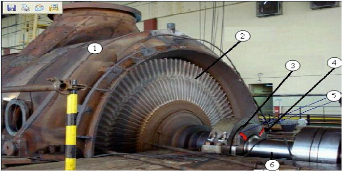
Fig.1 Low pressure turbine: 1) Housing 2) Rotor 3) Bearing 4) Proximitors 5) Amplifier 6) Shaft
2 LEARNING BY PROJECT
Laboratory work classes are an integral part of any educational program and their purpose is bringing the students closer to
37
ICERI 2012
real situations of the area of studies.
The methodology applied to present these mathematical tools, necessary to engineering professionals, not only the conventional ones but also state of the art monitoring rotating machinery, allow students to know that a large number of techniques are now available to use in vibration analysis so as to detect and diagnose incipient faults in operating machines. In addition, the fundamental purpose is to engage students in comparing these methods and analyzing their performance for each application.
3 SIGNAL ACQUISITION
The vibrations are measured in microns and should have the lowest values possible (ideally zero). The normal values for this kind of machine are round 30 to 40 microns.
As mentioned above, sensors will measure the variation of the magnetic field generating an electric signal that enters an amplifier from which a signal is obtained for an indicator, a recorder and a computer that saves the historical data.
38
ICERI 2012
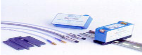
Fig.2 Proximity probe transducer
The orbit time base plots of the temporal signal from these proximitors are showed in Figure 3, obtained from different monitoring channels, captured at real time in determined radial and horizontal positions points.
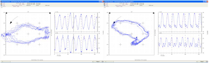
Fig.3 Orbit timebase plots
39
ICERI 2012
4 MODEL-BASED DIAGNOSIS
Since early 1980’s, various model-based approaches have been introduced to machine conditioning monitoring, mainly for the diagnosis of malfunctions in manufacturing and processing equipment. A number of parametric methods are available for modeling mechanical systems. These include autoregressive AR, autoregressive moving average ARMA, ARX with exogenous inputs, time –series models.
Autoregressive AR modeling stems from the demand for high-resolution spectral estimation. It belongs to the parametric modeling method with a rational transfer function. The AR model is appropriate for the estimation of spectra with sharp peaks but not deep valleys, which is the case for gear signals, and is particularly useful for modeling sinusoidal data. A deterministic random process is one that is perfectly predictable based on the infinite past. This means that a data sequence or discrete
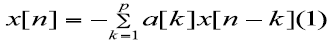
The data sequence may also be approximated using its finite (p)
40
ICERI 2012
preceding values. This model is expressed by a linear regression on itself (ie. autoregression) plus an error series of approximation.
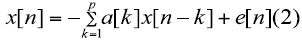
where e[n] is a Gaussian white noise series with zero mean and variance  and
and  the model order. The power spectral density (PSD) of the data sequence x[n] is:
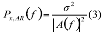
Were  represents the PSD of the AR coefficients, ie. a [n], n = 1, 2, ., p.
Since the estimation of AR parameters only involves linear equations, there are several wellestablished methods in estimating the AR coefficients, such as Levinson-Durbin recursion and Burg algorithm.
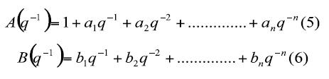
ARX model is an autoregressive model with exogenous inputs, these linear discrete time, single input/single output ARX model have the follow representation:
41
ICERI 2012

Where A y B are polynomials of order n in the backwards shift operator 
5 VIRTUAL INSTRUMENTS AND SIMULATIONS
Data acquisition by proximitors channels are considered to built off-line a parametric model by the LabVIEW software, to make a comprehensive analysis and processing of the signal, and displays the final calculation of test results.
The data samples and data samples reproduced using ARX time series models are matched in Figure 7, and the residual error is display in Figure 8. These figures show the capabilities to predict data from reference and damage conditions of the system.
42
ICERI 2012
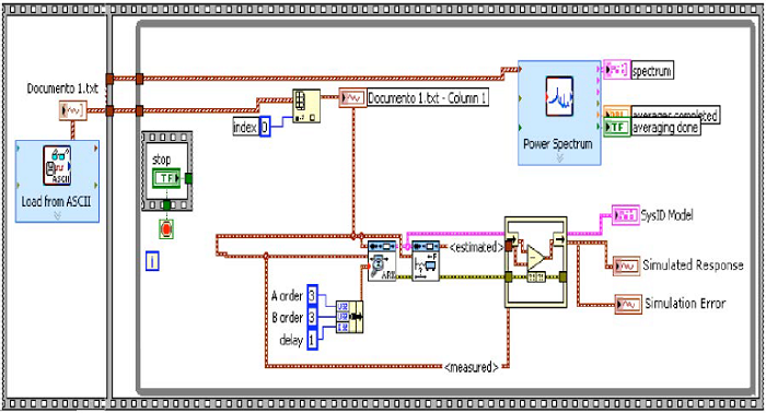
Fig.4 Block diagram
43
ICERI 2012
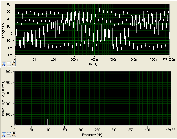
Fig.5 Channel 5 data signal and the power spectral density
These ARX models had been developed to predict the vibration responses of individual sensors basedon data from healthy conditions
44
ICERI 2012
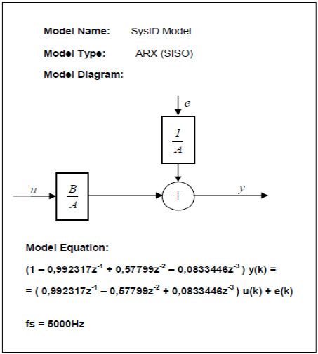
Fig.6 ARX Model
45
ICERI 2012
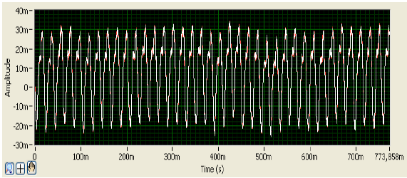
Fig.7 Model ARX and original signal
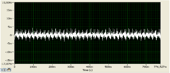
Fig.8 Residual error
46
ICERI 2012
6 FUTURE WORK: COMPARISON OF DIAGNOSTIC METHODS
This procedure for damage detection and localization within a mechanical system is solely based on the time series analysis of vibration signals. The standard deviation of the residual errors, which is the difference between the actual measurement and the prediction derived from ARX model, can be used as damage-sensitive feature to locate damage.
The premise of this approach relies on the fact that the residual error associated with ARX model, developed from data obtained when the structure is undamaged, will increase when this model is applied to data obtained from a damaged system.
To verify that one method is more useful than others, it will be necessary to examine several time records corresponding to a wide range of operational and environmental cases, a wide range of damaged and undamaged structures, as well as different damage scenarios.
The ability to perform damage detection in an unsupervised learning mode is very important as data from damaged structures are typically not available for most real-world
47
ICERI 2012
structures.
These approach presented is a based method for developing an automated continuous monitoring system because of its simplicity and its minimal interaction with users.
7 CONCLUSION
A fault diagnosis system which uses technological tools is considered a suitable way for project learning, these systems were developed by recent different virtual platforms and allow students to develop professional future works by analyzing their advantages in monitoring and diagnosis in realtime.
The experience acquire using virtual instruments leads engineering professional to a kind of learning
that is called learning by doing, i.e. learning with real problems.
Learning by doing is one of the universal forms of learning, is a more natural learning, and easier to link with objectives relevant to the learners, their interests and their motivation to learn, as well as having an immediate relationship with the trial- error- success cycle.
When using computers "learn by doing" becomes a powerful
48
ICERI 2012
strategy using simulations and other interactive forms, as simulations have always been seen as the most appropriate way to learn together with computers due to the high level of involvement that requires an action-oriented active learning.
ACKNOWLEDGMENTS
The authors would like to thank Apply Energy Support Company for the information submitted.
REFERENCES
1. Fernández, A., Bilbao J., Bediaga, I., Gastón A., Hernández, J.(2005). Feasibility study on diagnostic methods for detection of bearing faults at an early stage. WSEAS Int. conf. on DYNAMICAL SYSTEMS AND CONTROL, pp113-118.
2. Nour, A. , Chikh, N., Chevalier, Y., & Saci, R.(1989).Spectral Analysis and Autoregressive Model of a Rotor Vibratory Signal, ISMEP Paris.
3. Thanagasundram, S. & Soares Schlindwein, F.(2006). Autoregressive
49
ICERI 2012
Order Selection for Rotating Machinery. International Journal of Acoustics and Vibration. (Vol. 11, N° 3).
4. Randall Robert(2004).State of Art in Monitoring Rotating Machinery. Journal Sound and Vibration, pp 10-16.
5. Wenyi W. and A. K Wong(2000). A Model-Based Gear Diagnostic Technique. DSTO Defense Science & Technology Organization C. of Australia Dec.
6. Ho D. and Randall R. B.(2000). Optimization of bearing diagnostics techniques using simulated and actual bearing fault signals. Mechanical systems and signal processing, (Vol.14, Nº 5, pp.763-788).
7. Tinnirello, A.(2006). Stochastic Models in Engineering Quality Problems. Journal WSEAS TRANSACTIONS on SIGNAL PROCESSING. (Vol. 2, Issue 2).
8. Tinnirello, A., Dadamo, M., De Federico, S., Gago, E.(2008). Predictive Models to Monitor Feedwater Boiler in SteamTurbines. COMPUTATIONAL ENGINEERING IN SYSTEMS APPLICATIONS. 12th WSEAS, (Vol. 1, pp. 230-235), Greece.
9. Wang, W.(2008). Autoregressive model-based diagnostics for gears
50
ICERI 2012
and bearings. British Non- Destructived Testing and Condition Monitoring . (Vol. 50, Issue 8 pp. 414-418).
10. Wang, W & Wong, A.(2002). Autoregressive Model-Based Gear Fault Diagnosis. Journal of Vibration and Acoustics. (Vol. 124, Issue 2, pp. 172 -180).
11. Chen, Z., Yang, Y. M., Hu, Z. & Shen, G.(2006). Detecting and Predicting Early Faults of Complex Rotating Machinery Based on Cyclostationary Time Series Model. Journal of Vibration and Acoustics. (Vol. 128 Issue 5 pp. 666-672).
12. Zhan Y., Makis, V., Jardine, A.(2003). Adaptive model for vibration monitoring of rotating machinery subject to random deterioration. Journal of Quality in Maintenance Engineering. (Vol. 9, Issue 4, pp. 351-375).
51
EDULEARN 2013
INTERDISCIPLINARY ACTIVITIES TO IMPROVE THE LEARNING METHODOLOGY PERFORMED IN MECHANICAL ENGINEERING DEGREE STUDIES Descargar pdf
Alicia Tinnirello1, Eduardo Gago2, Mónica Dádamo2
1 Universidad Tecnológica Nacional. Facultad Regional Rosario (ARGENTINA)
2 Universidad Nacional de Rosario (ARGENTINA)
atinnirello@frro.utn.edu.ar, egago@frro.utn.edu.ar, mdadamo@frro.utn.edu.ar
Abstract. The multidisciplinary character of engineering studies should be considered, in the process of teaching and learning mathematics, as a key to ensure that students incorporate knowledge in a meaningful way so as to be used in the development of basic and applied technologies.
The current work describes methodological changes implemented in Advanced Computing at the Mechanical Engineering studies, which we believe to be innovative, aimed to integrate disciplines, with an approach based on the complexity of fluid flow systems and mathematical models, so as to introduce
53
EDULEARN 2013
small working groups of students in research work and to pursuit new knowledge.
The so-called virtual labs have emerged in the area of engineering education as a potential alternative to the traditional laboratories. This new learning system is possible due to the capability offered by the recent technological advancements that allow us to resolve symbolic and also numerically each system, which can be represented by a mathematical model and designed using simulation models, these present outstanding advantages in the process of teaching in several disciplines.
This change in the context of learning in Engineering aims to place emphasis on the interpretation of the various parameters of the systems under study, using tools of symbolic manipulation; and the generation of a field of collaborative work; allowing the formation of basic capabilities; having an impact in the student’s multidisciplinary formation.
This presentation includes the planning, analysis and selection of contents in the study of models
related with Fluids Mechanics, by employing a platform of multiphysics simulation where Mathematics and varied Physics systems can promote and facilitate the conceptualization of complex models.
54
EDULEARN 2013
Keywords: multidisciplinary, virtual labs, fluid flow, computational mathematics.
1 INTRODUCTION
In an age characterized by new dimensions of complexity, scale and uncertainty, many challenges require solutions that are beyond the reach of one thought discipline. More and more frequently, the advances in science and engineering that will have the greatest impact are those born at the frontiers of more than one engineering discipline. The benefits of multidisciplinary thinking - and the shortcomings of a world that has been “understood” primarily by specialization - have been apparent for several decades.
While the concept of multidisciplinary thinking, or “multidisciplinarity,” is not new, it has in recent years emerged as a pervasive term, gaining popularity both in science and in policy contexts. Multidisciplinarity traces its roots to the second
55
EDULEARN 2013
half of the 20th Century, with the cross-fertilization among the sub-branches of physics, the development of grand simplifying concepts, the emergence of systems theory and of new fields such as biochemistry, radio astronomy and plate tectonics.
Multidisciplinary engineering refers to engineering that engages one or more areas of engineering e.g. mechanical, chemical electrical, biomedical, etc.), as well as other sciences or technical isciplines. Multidisciplinary engineering often requires team work. For instance, a mechanical ngineer works with a biologist to design a heart valve. In this example, the teammates work together, ach contributing their own expertise to solving the problem. Multidisciplinarity additionally refers to he development of conceptual links using a perspective in one discipline to modify a perspective in nother discipline, or using research techniques developed in one discipline to elaborate a theoretical ramework in another.
In search of a multidisciplinary training the incorporation of technology in higher education allow significant changes in the teaching and learning process that impact on engineering careers, especially in the subjects of Mathematics area. The insertion of specific software and computational tools which are
56
EDULEARN 2013
increasingly powerful, allow making the modifications needed to achieve this purpose.
With the objective to carry out these changes we need to align the University curricula not only to the new work methods that allow intellectual development stimulation but also have a tendency to a multidisciplinary approach. The goal is not only to teach and learn only mathematics, is also doing it by facing with the stimulation of real cases and simple systems that lead the student to have a look at real situations.
The development of numerical methods and the advent of simulation platforms consider the need to guide the methodological approach of Higher Mathematics studies towards a new kind of teaching that modify the learning sequence. Driving the educational system approach to multidisciplinary models has an impact to the student’s cognitive process.
Multiphysics stimulation software create an engineering environment where learning opportunities and motivation increases exponentially. Moreover the comprehension improvement and ease of learning complex subjects are improved when trying to learn fluid flow processes with
57
EDULEARN 2013
educational purposes, processes that students could not observe and reason in the absence of these resources.
This paper recounts the experiences in Advanced Calculus class when analyzing the fluid flow from two different perspectives, the first aims to work by using mathematics software applying the subject of analytic functions of complex variables, and see the conclusions arrived, the second is to perform the same job but with a multiphysics simulation platform.
Currently, to run Applied Mathematics contents in Engineering studies in a significantly manner, it is convenient to enrich the teaching and learning process by implementing thematic oriented to present models that integrate different disciplines. But not only choosing these models is important, but also the means chosen for its resolution.
It is noteworthy that students are encouraged when they leave aside traditional forms of paradigmtype problem solving, and when they are imposed to a significant and reflexive learning dynamic that involves engineering situations which ignore ideality and are related to the ones to be carried out in practice. Sometimes it is observed that the students do not follow
58
EDULEARN 2013
abstraction and generalization processes, or find it difficult to adapt to them. This is why the trend in contemporary education needs the implementation of a system that places the student in centred processes that identify him as an active and reflective learning subject.
To carry out these changes that aim at leading the acquisition of new ways of thinking and reasoning, it is necessary for the teacher to reformulate the methods implemented in the class and is adapted to work in other areas where available modelling and simulation are applied [5].
2 APPLIED METHODOLOGIES
This engineering analysis work is based on a design and planning computer aided system. It is important to create a learning space at the higher education system where developed a set of activities and communicational expressions as the fundamental line of the educational process. It will organize theoretical and practical activities where students perform technological applications with the topics developed in class, linking the themes of the subject, in different subjects of
59
EDULEARN 2013
the same or different levels of the area, as well as with other disciplines through solving projects whose complexity is conditioned only by the basic knowledge that students have. Teaching strategies are established based on different practical activities without neglecting the theoretical foundation, with a multidisciplinary approach.
In the areas of professional cycle and following a multidisciplinary line, training activities are proposed, with a strong focus on professional activity carried out, showing industrial applications, designing projects with clear goals and objectives that allow the continuous update and coordination of activities in the areas of knowledge of the university studies. It is essential that students, from initiation to completion of their studies in their chosen field make use of computational methods. This will strengthen the student’s unified vision between mathematics and its applications and will give the essential tools for their professional work.
“When students learn in the same way they will act as Engineers, in their professional development, they will acquire a real meaningful learning.” Activities involved in this project include training teachers to implement the project in Basic
60
EDULEARN 2013
Sciences in Chemical, Mechanical, Civil and Electrical majors, conducting interdisciplinary workshops with the use of specific software and tailor-made training materials, training scholars in teaching and researches activities, developing teaching materials in electronic format to implement whether dual or distance education.
It is also intended to support planning and implementation of curricular activities to develop dual and distance learning through the institutional web site. This involves training teachers to develop activities suitable for distance learning and the ability to access materials and resources with the state of the arttechnology and bibliographical material as well as scientific publications throughout the working team[10].
3 TEACHING STRATEGIES
To improve their learning experience students need to have sufficient prior knowledge from which to address the content proposed, in order to establish more complex and rich relations. Therefore, it is initially convenient to help the student to remember, rearrange or assimilate their prior background
61
EDULEARN 2013
related with the new content, in order to successfully address the learning program, designing cognitive bridges between the new content and structure of knowledge that the student has - advance organizers - for that purpose appropriate strategies are developed to place students in a favorable position to learn. This involves an intense activity by the student and a real commitment of teachers in regard to the directionality, coordination and learning support.
In this regard, an integrated learning is developed - theoretical and practical and theoretical technology - in an attempt to differentiate experience based on: dialogue, convergence criteria and active student participation. We must ensure that students leave their passive role, acquiring memory ability that prevents think for themselves and create. The right and properly sequenced questions guide the student’s thinking through an argument that allows to reach certain conclusions, convergent thinking, thus a more dynamic and participatory exposure is performed.
The practical work-integrated projects of the units of the various agenda items must contain not only implementation but also activities of analysis and discussion, tending to integrate the
62
EDULEARN 2013
theoretical and practical, so proceed from reflection to action and then the improvement of the action. The teacher acts as a facilitator of learning “, leading to questions, presenting situations, pointing out mistakes and avoiding address what the student can solve by themselves. The situations should be simpler in the first stage gradually increasing its complexity [10].
4 PROJECT PLANNING
Project based learning has proved to be a suitable method to demonstrate the need of mathematics in professional engineering. Students are confronted, complementary to their regular courses, with problems that are of a multidisciplinary nature and demand a certain degree of mathematical proficiency [2].
The curricula of the Mechanical Engineering programs at our university include Advance Calculus at the third year of the engineering career; the authors’ experience is that students increased their interest and their appreciation for the contents if they are involved by learning in an applied way.
The project proposal was a selection of contents related with
63
EDULEARN 2013
Mechanics Fluids, by employing a platform of multiphysics simulation where Mathematics and varied Physics systems are involved to model the system behavior.
The simulation of different fluid behaviours is a technique widely used in the majority of the industries, being the computational fluid dynamics (CFD) one of the techniques that uses numerical methods and algorithms to replace the partial differential equation systems into algebraic equation systems to be resolved by the aid of computers.
CFD techniques provide qualitative and quantitative information about fluid flow prediction by means of resolving fundamental equations, allow predicting or simulating behaviours in a virtual laboratory.
Using CFD is possible to build a computational model that represents a system to study, specifying the physical and chemical fluid conditions of the virtual prototype and the software will deliver a prediction of the fluid dynamic, therefore is a design and analysis technique implemented by a computer. The main advantages are:
• Predicts the fluid properties with great detail in the studied domain.
64
EDULEARN 2013
• Helps design and prototype with quick solutions avoiding costly experiments.
• Process visualization and animation can be obtained in terms of the fluid variables [9].
The proposal presented is intended to explore potential theory examples and discuss some fluids that can be approximated using Computational Fluid Mechanic. When the potential flow presents complicated geometries or unusual current conditions, the conformal transformation based in complex variables cease being useful to generate forms of bodies. In this case the numerical analysis technique constitutes a more appropriate approach.
The finite difference method for the potential flow has the aim to approximate partial derivatives listed in a physical equation by “the difference” between the values of the solution in a number of modes spaced by some certain finite distance. The original equation in partial derivatives is replaced by a series of algebraic equations for the nodal values.
The system being studied is the two-dimensional flow of an incompressible fluid, non-viscous corresponding to an irrotational field that moves in a steady state for different values
65
EDULEARN 2013
of the potential velocity complex. Using complex function models, an analysis of the behaviour of the fluid is done to conceptualise the subject and then is contrasted with the introduction of CFD technique:
4.1 1st Session: Theoretical research of the topic
Groups of four students were formed with the suggested bibliographic material ([4], [6], [7], [8], [12]) and with an accompanying teacher, we came to understand and obtain a tutorial guide of theoretical concepts used in the proposed work, upon request, after hearing and reviewing the conclusions reached by each group, a debate about the subject took place proposing the following framework:
(i) A complex variable function 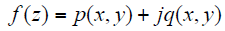 univocal some region R of the plane z , is analytic in the region R if a derivative f'(z) exists at every point z in that region R.
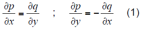
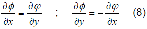
(ii) A necessary condition for that f(z) is analytical in a region R , is that in R , p and q satisfy the Cauchy-Riemann equations.
66
EDULEARN 2013
If these partial derivatives are continuous in R , then the above equations are sufficientconditions to be f(z) analytical in R. The functions that satisfy the above conditions are said conjugate and such functions satisfy the orthogonality property means that the type curves 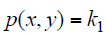 , and
, and 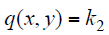 , are orthogonal.
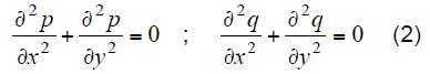
(iii) In addition if the second partial derivatives p and q are continuous in R, and Laplace equation is meet for p and q:
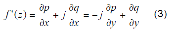
(iv) The derivative of the function f can be calculated by the following expression:
4.2 2nd Session: Modeling the system
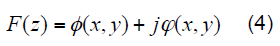
The velocity complex potential F is an analytical function of complex variable composed of the ordered pair whose real part is the velocity potential and imaginary part is the current
67
EDULEARN 2013
function  :
:
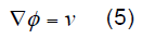
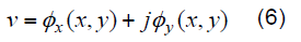
The fluid flow velocity is  , is the gradient of the potential velocity :
From equations (4) and (5) we could express that the fluid velocity in the Eq. (6):
Differencing the complex potential from Eq. (4) was obtained Eq. (7):
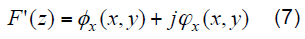
As F is an analytic function meets the conditions expressed by the Cauchy-Riemann equations it can be concluded that:
68
EDULEARN 2013
In this case the equipotential curves are those such that: 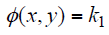 , and are orthogonal to the streamline which are equation curves
 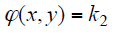 , (with k1 y k2 constants).
With the model accomplished and by Eq. 7 and Eq. 8 it could be concluded that the fluid velocity is a conjugated complex, derivate from the F function.
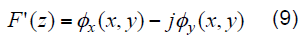
It expresses Eq. (9) also by means of Eq. (10):
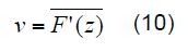
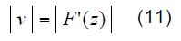
In order to calculate the magnitude of the velocity  was used Eq.(11).
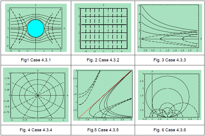
4.3 3rd Session: Analysis and discussion of different cases
4.3.1 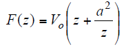
69
EDULEARN 2013
We propose to study the movement of a known fluid, for different expressions of the complex potential, considering in every case the constant  . Where
  is a positive constant.
We guide the students work analysis with the following instructions ([1], [3], [11]):
a) Obtain the equations for the streamlines and equipotential lines.
b) Make a graphical representation of the previous paths and interpret them physically.
c) From the graphs obtained in the previous section, discuss how the fluid regime is.
d) Analyse how the velocity profile will be at different points of his path.
e) Individualize the stationary points.
From the proposed analysis and by the graph of Fig. 1 the following findings were established:
(i) The axis parallel curves indicate paths that fluid particles follow. If  the path which moves in the x axes, or in the contour of circle of radius a.
(ii) Equipotential lines are marked with dotted lines and are orthogonal to the streamlines.
70
EDULEARN 2013
(iii) The circumference of radio a represents a path, and since there can’t be a flow through a path, it can be considered as a circular obstacle of radius a placed in the fluid path.
(iv) The complex velocity of the fluid has a variable value near the obstacle and its modulecorresponds to 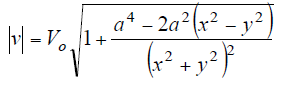
(v) If we move away from the obstacle the velocity takes the value  , i.e. the fluid is running on the positive x axis direction with constant velocity
  .
.
(vi) The stationary points of the system are those where the velocity is zero and are given by the values of  and
and  .
.
4.3.2 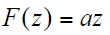
From the analysis of Fig. 2 we been able to visualize the behaviour of the fluid in this case, where the power lines are horizontal lines and the corresponding equipotential curves are vertical lines, indicating that the fluid flow is uniform and its direction is right, this is also interpreted as a uniform flow in the upper half plane bounded by the x axis, which is a streamline, or
71
EDULEARN 2013
a uniform flow between two parallel lines  and
and  , with its velocity
  , and its module of the same value.
4.3.3 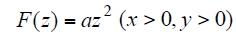
From observing Fig. 3, we see that the fluid is forced to rotate towards a corner located at the origin. In this case, the streamlines are branches of rectangular hyperbolae responsive to the equality  , so that the velocity module is directly proportional to its distance from the origin, being its expression
  . It was concluded that the value of the stream function at a point is interpreted as the flow rate through a line segment that joins the origin with that point.
4.3.4 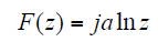
Streamlines analysed in Fig. 4 are circles having a common centre which corresponds to the origin of the complex plane ( ) while the equipotential lines are given by the lines of equations
  , which also pass through the origin. Thus the complex potential describes the flow of a fluid that is circling around is called “vortex” and this type of flow is called “vortex
72
EDULEARN 2013
flow”. In this case the direction flow matches clockwise direction and the magnitude of the velocity is: 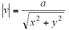
4.3.5 
As shown in Fig. 5, we study the region in the first quadrant, in this case we observed that the streamlines for this region are bounded by the x axis and the line  . The direction flow is downward and the value of the module of the velocity is
  .
.
4.3.6 
In this case Fig. 6 shows that the streamlines are concentric circles around a point and that from that point equipotential curves are born. It appeared that the velocity module corresponding to the formula is: 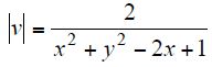
73
EDULEARN 2013
5 THE IMPACT OF APPLYING CFD TECHNOLOGY
Taking the proposal of work done in section 4.3.1 the simulation is performed with the Creeping Flow module of COMSOL Multiphysics. The working environment of the
74
EDULEARN 2013
program allows adding to the proposed model, new physical parameters besides proposing, evaluating and exchanging boundary conditions. The potentiality that the program has, contributed to work with educational proposals that approximate to reality aside from the ideal conditions.
5.1 Simulated domain and physical conditions
By 6 cm diameter UNS C10100 bronze pipe, water flows in a laminar regime with a Reynolds number less than 2500 and a temperature of 20 ° C. In this pipe there is a blockage of a sphere of alloy steel 1006 (UNS G10060) of 0.3 cm radius. If the pressure ranges from 3 to 2 Pa in a section of 10 cm length, and it is considered that the fluid has viscosity on the outer walls and roughness in the sphere, it is requested to study the variations in the pressure and velocity caused by such obstruction.
Using conformal mapping techniques based on complex variable techniques there are no friction losses and the fluid is considered in ideal conditions, with COMSOL platform is not possible to consider the value of zero viscosity.
75
EDULEARN 2013
5.2 Prototype Geometry and Meshing
As shown in Fig. 7, tools that the program has to perform rendering of geometry working are used. However, we must note that the software allows importing models with more complex designs from design programs in solid such as Solid Works, Space Claim and Inventor. This interaction between programs is very useful for the design of complex geometries.
The procedure for performing the profile graph of the shape of the pipe is: define the dimensions of the rectangle, the size and position of the sphere, and use the intersection tool to complete the geometry. Choosing a correct meshing is of utmost importance to verify the accuracy of the results. To make the mesh, it is taken into account the shape and the maximum and minimum measurements of geometry to study. Prior to making the modeling, we proceed to the meshing of the geometry used, to visualized in Fig. 8, the standard predefined triangular free mesh made automatically has been opted.
76
EDULEARN 2013
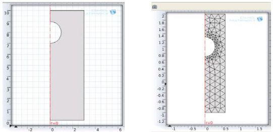
Fig.7 Prototype Geometry
 Fig.8 Meshing
5.3 Results
Fig. 9, Fig. 10 and Fig. 11 shown the formation from the tube walls of a profile with increasing velocity called boundary layer. In the central part, where the sphere is positioned, zero velocity are noticed at the front and rear of it, indicating the absence of fluid flow in that area and as a result of this, significant pressure fluctuations.
Fig. 12, Fig. 13 and Fig. 14 show that at the side of the sphere there is a considerable pressure drop which results in an
77
EDULEARN 2013
increase in velocity due to the decreased cross-sectional area. This situation is similar to what occurs in other measuring instruments such as flow rates and Venturi tube, nozzle and orifice plates.
In the front of the sphere the absence of velocity causes the maximum pressure in this area, because of this it can be understood the basis of certain measuring instruments that use stagnation of fluids, such as the Pitot tube used to measure total pressure and the Prandtl tube used for measuring dynamic pressure and velocity.
At the rear of the sphere there is a low pressure zone, which can cause the detachment of the boundary layer. This may happen or not depend on each case from the fluid conditions and roughness of the sphere.
Even though graphics of pressure and velocity have been made over time, the program also allows evaluating specific points or features of the model and finding the maximum and minimum values of both velocity and pressure.
As for the model used, as long as the student acquires greater expertise a higher degree of problem complexity could be achieved, varying border conditions or using this model as a
78
EDULEARN 2013
starting point for studies in nozzles, diffusers or in other engineering applications.
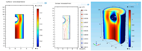
 Fig.9 Velocity level
 Fig.10 Velocity level
Fig.11 3D velocity level
Fig.10 Velocity level
Fig.11 3D velocity level
 surfaces
curves
surfaces
surfaces
curves
surfaces
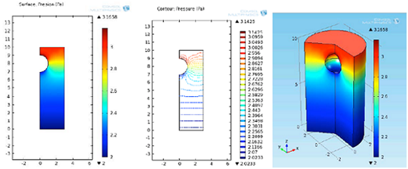
Fig.12 Level pressure
Fig.13 Pressure level
Fig.14 Level pressure
surface
curves
surfaces
79
EDULEARN 2013
In Fig. 15 and Fig. 16 depicts graphs of the level surfaces corresponding to the velocity and pressureof each level.
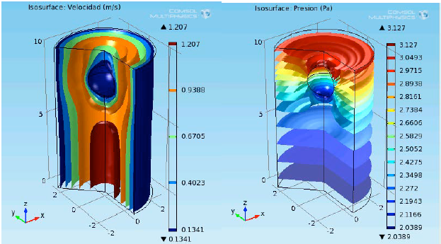
 Fig.15 Velocity level surfaces
 Fig.16 Pressure level surfaces
Besides the above, the narrowing of sections, such as the one caused by the sphere, are the basis of some instruments operation such as ejectors, used to mix fluids and accelerate fluids.
The observed variations also allow to understand why we recommend placing the measuring instruments to 5 times the
80
EDULEARN 2013
minimum diameter of the pipe, from any disturbance so as to achieveresults biased by them.
6 CONCLUSIONS
The use of analytical functions of complex variables, the study of idealized models and support of computer resources used appropriately lead to a contextualized analysis which achieve the goal of understanding the possibilities of integration between computational mathematics and fluid mechanics.
These laboratory experiences are a link between basic science and applied technologies that equip students an autonomous character to work with problem situations similar to their future professional work.
Through numerical simulation and basic knowledge of fluid flow simple problems are introduced using an environment such the one offered by COMSOL platform to assess the importance of the results obtained in an analytical and symbolic form, and the possibilities for future use of the virtual learning laboratory, in applied technologies studies, to support disciplinary integration activities.
81
EDULEARN 2013
This methodology allows deepening and integrating the basic concepts, as well as arousing student interest in the incorporation of new topics, to be able to show from the early years of their careers and present practical applications of recent development work which may lead to a constant search for new knowledge.
The intense activity has also allowed the incorporation of young students for training in both teaching and research, who work on activities that are carried out in the laboratory and approaching concerns and addressing engineering problems in the subjects of upper cycle.
ACKNOWLEDGMENTS
The authors would like to express their recognition to their students Carlos Tosoratto and Mariano Valentini for their performance during their project work development.
82
EDULEARN 2013
REFERENCES
1. Bird, R.; Stewart, W.; Ligthfoot, E. (2007). Transport Phenomena. Wiley & Sons Inc. 2nd. Ed.
2. Bischof; G., Bratschitsch, E.; Casey, A.; Rubesa, D. (2007). Facilitating Engineering Mathematics Education by Multidisciplinary Projects American Society for Engineering Education.
3. Cengel, J.; Cimbala, J. (2006). Mecánica de Fluidos: Fundamentos y aplicaciones. México. 2ª Ed. Edit. McGraw-Hill.México.
4. Churchill, R. (2004). Variable compleja y Aplicaciones. McGraw Hill, 7ª Ed.
5. Gago, E.; Dádamo, M. et al. (2010). La Importancia del Enfoque Multidisciplinar en la Enseñanza en Ingeniería Mecánica. II CAIM - Segundo Congreso Argentino de Ingeniería Mecánica. San Juan, Argentina.
6. James, G. (2002). Matemáticas Avanzadas para Ingeniería, Prentice Hall, 2ª Ed.
83
EDULEARN 2013
7. Ledder, G. (2006). Ecuaciones Diferenciales, un Enfoque de Modelado, Mc Graw Hill.
8. O´Neil, P. (2004) Matemáticas Avanzadas para Ingeniería, MathLearning, 5ª Ed.
9. Orrego, S. (2009). Simulación de Fluidos utilizando computadoras. Universidad EAFIT. Medellín. Colombia. http://mecanica.cafit.edu.co
10. Tinnirello, A.; Gago, E.; Dádamo, M. (2010). Designing Interdisciplinary Interactive Work: Basic Sciences in Engineering Education.The International Journal of Interdisciplinary Social Sciences. Vol. 5, F. 3, pp. 331-334. Cambridge.
11. White, F. (2004). Mecánica de Fluidos. Mc Graw Hill 5ª. Ed.
12. Zill, D.; Cullen. M. (2002). Ecuaciones Diferenciales con problemas de valores en la frontera, Thomson Learning, 5ª Ed.
84
ICERI 2014
DESIGN, SIMULATION AND ANALYSIS OF A FLUID FLOW SYSTEM THROUGH MULTIPHYSICS PLATFORM Descargar pdf
Alicia Tinnirello, Eduardo Gago, Mónica Dádamo, Mariano Valentini
Universidad Tecnológica Nacional (ARGENTINA)
Abstract. The demands in the field of Engineering Education stand out as skills and attitudes required by the future engineer, assume a mental framework of behavior that facilitate them to operate in an environment of high mobility, in terms of knowledge and technologies. We are convinced that the knowledge about the educational reality engineering must be closely linked to the determinants -everchanging and situational - of the action, and that the only way to establish a rational control is on the same multidisciplinarity.
The curricula of the Mechanical Engineering programs at our university include Advance Calculus at the third year of the engineering career, the authors experience is that students
85
ICERI 2014
increased their interest and their appreciation for the contents if they are involved by learning in an applied way. The project proposal was a selection of contents related with Fluids Mechanics, by employing a platform of multiphysics simulation where Mathematics and varied Physics systems are involved to model the system behavior. We present a simulation performed by a multiphysics platform for designing and analyzing the behavior of industrial equipment. This simulation is carried out by applying the CDF and the technical module of creeping Flow of Comsol component that allows not only to build a computational model that represents the model to study by specifying the fluid physical and chemical conditions, but is also accessed information of the corresponding system velocities outlines and temperature gradients plotted in 3D.
This change in the context of learning in Engineering aims to put the emphasis on the interpretation of the various parameters of the systems under study, using the tools of symbolic manipulation; and the generation of a field of collaborative work; allowing the acquisition of capacity and impacting in the multidisciplinary student training. The advantages by using this kind of platform are centered in the difficulties presented by the
86
ICERI 2014
conventional analytical methods to analyze complex geometries and to solve nonlinear systems.
Keywords: Multidisciplinarity, simulation, fluid flow, technology.
1 INTRODUCTION
The technological resources provide a broad possibility of representation and calculation allowing to incorporate fundamental changes in how to teach. For more than two decades, in the academic field, the potentialities offered by the technology affects the activities that are derived to the classroom’s area. Under the experiences which have been developed in engineering careers, are then installed the need to develop methodologies for teaching and implementing the interaction between the different areas to enhance the student's ability in the acquisition of concepts and its further use in the models required for the resolution of engineering problems.
87
ICERI 2014
The current trend in the learning process of Mathematics relevant to the basic technologies and aims to bring students to the modeling and simulation of real-life situations. The majority of which are not in the textbooks but come from the search for examples that come from the investigation of the teachers and that they are accompanied by interest and motivation of the students. [1]
In the context of meaningful learning, the students' activities must be oriented in a school system based on research and development of appropriate strategies for connecting and integrating the computational mathematics and the basic technologies and applied in Engineering to promote the multidisciplinary approach to the curriculum content corresponding to the plans of study, aiming to train professionals capable of solving complex models with the use of technologies.
The existence of simulation tools transformed the programming environments toward more collaborative spaces, with the updated listings of increasingly complex systems but with broad application in the various areas that comprise the engineering, it is possible to design methodological strategies
88
ICERI 2014
that integrate the knowledge of the compartmentalized disciplines.
The developments that have experienced the mathematical software and the affinity that the students have to be linked with the technologies, imposes on the university teachers makes the effort to transform the teaching-learning process in the process of learning investigating.
In the areas of engineering education have emerged a potential alternative to the traditional laboratories, the so-called virtual labs. This new system of learning is possible given the capacity of the recent development of technologies that allows you to resolve each system symbolic and numerically, which it can be represented by a mathematical model and designed using simulation models. [1]
2 OBJECTIVE
The proposal aims to show the consequences of the provision of a current of air stream than enters a fluidized bed dryer using the theory of the Computational Fluid Mechanics.
Through the analysis of the proposed system is intended to
89
ICERI 2014
show the advantages of using a multiphysics platform simulation, pointing out first that such software do not replace the experience and knowledge of the engineers, but they come to be an additional tool that saves time that would mean the cumbersome process of manual calculations.
This simulation is carried out by applying CFD technique, and the use of the module of creeping Flow of COMSOL, component which allows not only to build a computational model that represents the system to study by specifying the physical and chemical conditions of the fluid. It is also accessed graphics that analyze the profiles of speed and temperature gradients in the entire system. [2] [3]
The study of flows in a fluid into the dryer can be analyzed in different ways, taking into account what are the parameters (temperature, velocity, density or flow) that vary in the inlet of the dryer and what are the requirements to obtain as a result of the transformations that suffers the fluid, which should be done inside the dryer is to get a temperature constant output, since the moisture of grain to dry is a function of temperature. [2]
90
ICERI 2014
3 DESCRIPTION OF THE PROCESS
The fluidized bed dryer consists of a system where the particles are partially suspended in a gas stream ascending. The particles are lifted and then fall at random so that the resulting mixture between solid and gas acts as a boiling liquid. The contact is established between the solid and gas is the adequate to make it a better mass transfer between the two.
The fluidized bed dryer works with the condition that the air’s velocity is greater than the speed of sedimentation of the particles that float partially suspended in the flow of gas (The resulting mixture of solid-gas behaves like a fluid, which is why it is said that the solid are fluidized).
This technique is very efficient for drying granular solids, because each particle is completely surrounded by gas. This equipment is projected to analyze the output of the fluid under different conditions of entry of the hot air, determining the relationships between the input and output of the fluid’s parameters. The implementation of fluidized beds to a dryer of solid particles represents an approach to the problem of increasing the speed of heat transfer between the walls and currents of the process.
91
ICERI 2014
The product is fed by the upper part of the team through a tilted trough. To inject it with a fan inside the drawer of blowing, the processed air (hot or cold) are distributed in a homogeneous way thanks to the solera perforated prepared in the bed, occur the fluidizing product. The top of bed is composed of a campaign which aims with a removal fan; the contaminated processed air with fine of the product, which in addition is responsible for balancing the pressure within the fluid bed.
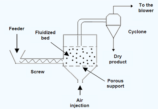
Fig.1 Process scheme.
92
ICERI 2014
4 APPLICATION OF CFD TECHNOLOGY
The simulation is performed with the Creeping Flow module of COMSOL Multiphysics. The working environment of the program allows adding to the proposed model, new physical parameters besides proposing, evaluating and exchanging boundary conditions. The potentiality that the program has, contributed to work with educational proposals that approximate to reality aside from the ideal conditions.[4]
Using CFD is possible to build a computational model that represents a system to study by specifying the physical and chemical conditions of the fluid to the prototype virtual software delivery and the prediction of the dynamics of the fluid, Therefore, it is a design technique and analysis implemented in a computer. The main benefits of using this technology are: the prediction of the properties of the fluid with great detail in the domain studied the design and prototyping of the computer while avoiding costly experiments, and the visualization and animation of the process in terms of the variables. [3]
Using the simulation with the COMSOL software will play that happens with the flow of fluid within the grain dryer. It is
93
ICERI 2014
estimated a density of grains constant inside the dryer that enters a constant temperature. Then, it should be assessed under different temperatures of entry and under different speeds of income in the fluid’s air heater.
5 SIMULATION METHODOLOGY
The simulation of the behavior of different fluids is a widely used technique in most of the industries,
being the dynamics of computational fluids technical CFD that use numeric methods and algorithms to
replace the systems of differential partial equations in algebraic systems of equations to solve by
means of the use of computers.
CFD techniques provide qualitative and quantitative information of the prediction of the flow of fluids
through the solution of the fundamental equations; it can predict or simulate behaviors in a virtual
laboratory.
Using the simulation with the COMSOL software will play that happens with the flow of fluid within the
grain dryer. Then should be assessed under different entry temperatures, and above of different
velocity of income in the air heater the fluid.
94
ICERI 2014
Using CFD is possible to construct a computational model representing the grain dryer to study the
physicochemical specifying air conditions assumed in the virtual prototype and the software supplied
predicting fluid dynamics, therefore, it is a design technique and analysis implemented in a computer.
The main advantages in using the CFD technique are that fluid properties are predicted in great detail
within the domain of the system studied, collaborates with the design and prototyping through the
possibility of quick solutions avoiding costly and risky experiments, and the possibility of obtaining the
display and animation of the process in terms of the variables in the fluid.
By means of the simulation with the software COMSOL will reproduce that it happens to the flow of the
fluid inside the dryer of grains. Constant density within grains entering the dryer at a constant
temperature is estimated. Different temperatures of heating element are then evaluated, keeping the
velocity of incoming air.
95
ICERI 2014
6 PROTOTYPE OF GEOMETRY
COMSOL simulation platform allows the prototype of the system shown in Fig. 2
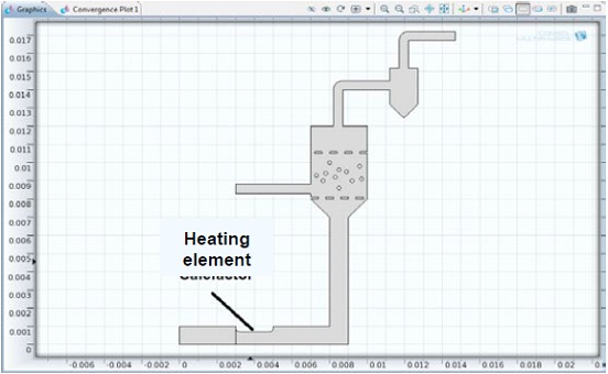
Fig.2 Geometry of the equipment.
7 SIMULATION AND PHYSICAL CONDITIONS OF DOMAIN
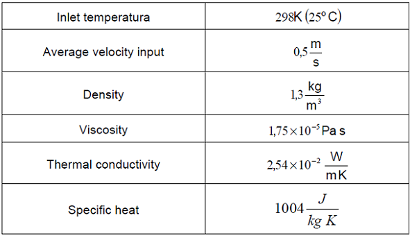
The fluid that enters through the pipe is air at atmospheric pressure, and the analysis is performed in a steady state, with a
96
ICERI 2014
flow which is considered incompressible. Furthermore, the pressure drops and
temperature variations are neglected. Constant density within grains entering the dryer temperature
constant is estimated 293 K (20°C), and considering the thermal conductivity of the heating element

The values of the physical conditions of the air selected to make the experience are set forth in the
following table:
Table 1. Physical properties of air.
97
ICERI 2014
8 MODELING SYSTEM
The process is carried out for a modeling using COMSOL Multiphysics defined through the following
steps: creating a geometry creating a mesh, a physical specification, the choice of solution and
visualization of results.
In the study of fluid flow is important to consider the assumptions about the density variations to
changes in pressure and temperature. The software application module is for incompressible fluids
are, however, allowed small changes are motivated by variations in temperature density. [4]
The Navier-Stokes equations are used by the program to model COMSOL phenomena that are
related to the heat transfer, considering that the density is constant in making the convective term. The
convective term in the Navier-Stokes 
98
ICERI 2014
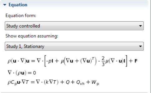
Fig.3 Navier Stokes equations.
9 ANALYSIS AND RESULTS
COMSOL provides the results is by the appearance of an image showing the model solution based on
each requested parameter.
At this stage certain subfolders that help the user to interpret the results from different representations,
ie, a graph showing a figure with a legend or just a table with the values corresponding to the desired
result is. The software allows the
99
ICERI 2014
display of the values of the parameters studied, showing graphs with
different shades of colors.
Dryer analysis considering the temperature of the heating element with values of 700 K. In Fig. Four is
performed, one can appreciate the level surfaces for the velocity profile of the fluid, while in Fig. 5
shown temperature gradients.
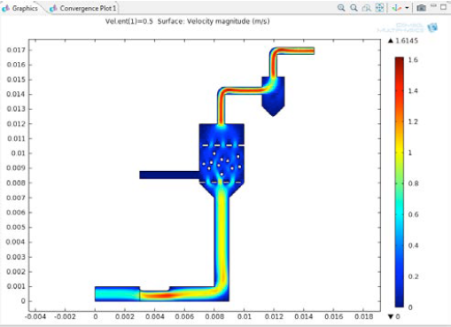
Fig.4 Velocity profiles.
100
ICERI 2014
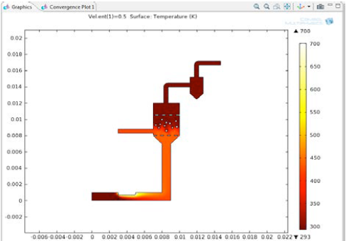
Fig.5 Temperature gradients.
In the Fig. 6, it is seen that as the velocity of air entering the dryer is increased, the outlet temperature of the air is increased first in a linear fashion, to about 1 m / s, and then begins to stabilize at a constant value, meaning that even if the input speed is increased not achieved that the outlet temperature behaves linearly. [5],[6]
101
ICERI 2014
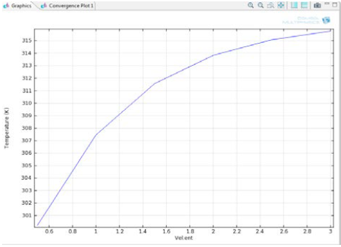
Fig.6 Outlet air temperature in the cyclone.
A reverse situation occurs with the density of air at the outlet of the cyclone, as it decreases indicating that the fluid is expanded by increasing the temperature. If different inlet air velocities are analyzed, it is possible to find the relationship between these and temperature output, allowing you to adjust the dryer to the requirements of the grains to dry and to variations in temperature and battery charge.
102
ICERI 2014
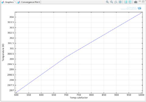
Fig.7 Outlet temperature based on the temperature of the heating element.
In the Fig. 7, considering the rate of air intake of 0.5 m / s, and the heating element temperature is
varied, the outlet temperature has a linear relationship with the temperature of the heating element,
i.e, it is constant if the input speed is achieved to adjust the cyclone outlet temperature by adjusting
the temperature of the heating element.
After this analysis, it was decided to reduce the temperature of the heating element to fifty percent to
see what happens to the
103
ICERI 2014
speed output parameters and temperature. Also observed this, one proceeds
to a comparison if halve the spaces through which air flows in the area of the fluidized bed of the
dryer. [5],[6],[7]
The Fig. 8 and Fig. 9 show the activity of the dryer when the heater temperature is 350 K, this
reduction in the heating temperature does not present a significant variation in the parameters
analyzed in the area of the fluidized bed.
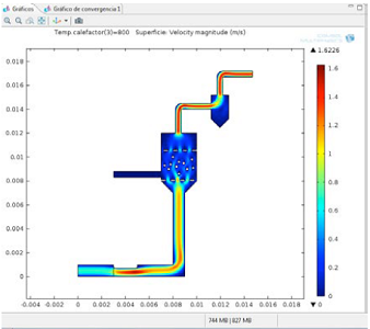
Fig.8 Velocity profiles.
104
ICERI 2014
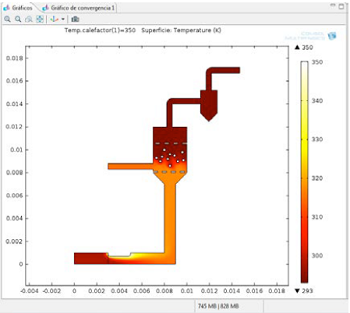
Fig.9 Temperature gradients.
In the Fig. 10, it is noted that as the velocity of air entering the dryer is increased, the outlet air
temperature is always increases linearly shaped but with two straight sections that have different
slopes. Accordingly, if the input speed to be increased is achieved that the outlet temperature behaves
linearly, but with temperatures lower than those obtained with a heating temperature to twice its output
value.
By reducing the temperature of the heating element slowing dryer process is obtained, as
temperatures exiting the cyclone
105
ICERI 2014
are much lower, indicating that in the fluidized bed heat losses occurs, which results in preservation of product quality, in reducing treatment times, and reducing energy consumption. [6]
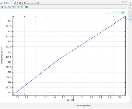
Fig.10 Temperature gradients.
If also discusses the fact reduce the area of the slots through which the air in the fluidized bed, leading to double spaces through which the air, it is seen that no significant changes
106
ICERI 2014
occur in the drying process, as the temperature is maintained at the same values. However, the risk of increasing the pressure of the circulating air is run, which could alter other parameters of the dryer. The Fig. 10 and 11 show the temperature within the fluidized bed when the number of slots through which the air is changed.
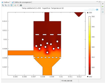
Fig.10 Temperature within the fluidized bed.
107
ICERI 2014
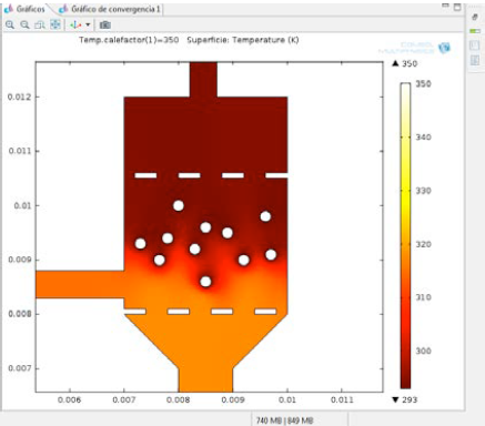
Fig.11 Temperature within the fluidized bed.
10 CONCLUSIONS
The use of a work environment with a multiphysics simulation platform is suitable for solving systems of fluid flow in which geometry of the problem difficult to resolve by conventional analytical methods. As the treaty system, it could be more complex further study done by the analysis of other parameters,
108
ICERI 2014
such as analyzing the fluid outlet when changes occur in the grain size study are planned in future
research.
The use of COMSOL in the analysis of parameters of a unit shows the importance of the
implementation of technologies for the study of major phenomena that occur in the nature of fluid flow
and heat transfer in a given context.
From the results obtained in the simulation can effectively analyze the behavior of the fluid under
different conditions and comprehensively analyze the behiavor of its path. It follows that the use of the
virtual platform streamlines the combined study of physical phenomena, contrasting the methods used
to verify the experimental results.
It is of great importance to computer application in solving fluid flow systems, where due to the
geometry of the model is very complex resolution by conventional analytical methods.
REFERENCES
1. Tinnirello, A.; Gago, E.; et al. (2013). Interdisciplinary activities to improve the learning methodology performed in mechanical engineering degree studies. EDULEARN 2013 (pp. 5407-5416).
109
ICERI 2014
Barcelona.
2. Cengel, J.; Cimbala, J. (2006). Mecánica de Fluidos: Fundamentos y aplicaciones. México. 2ª
Ed. Edit. McGraw-Hill.México.
3. Torres, R; Grau, J. (2007). Introducción a la mecánica de fluidos y transferencia del calor con
Comsol Multiphysics, Barcelona. Addlink Media.
4. Comsol. Introduction to CFD (2011). Módulo, versión 4.2a.
5. Alhama, F.; Madrid, C. (2012) Análisis dimensional discriminado mecánica de fluidos y
transferencia de calor. Edit. Reverté. Barcelona, pp. 235-239.
6. Geankoplis, C. (1999). Procesos de transporte y operaciones unitarias. Edit Cecsa, México. pp.
775-812.
7. Bird, R.; Stewart, W.; Ligthfoot, E. (2007). Transport Phenomena. Wiley & Sons Inc. 2nd. Ed.
110
CADI 2014
INTEGRACIÓN DE CONCEPTOS EN EL ANÁLISIS DE LOS MÉTODOS NUMÉRICOS: VINCULACIÓN MATEMÁTICA-INFORMÁTICA Descargar pdf
Mónica Dádamo1, AliciaTinnirello2
Laboratorio Multidisciplinar de Ciencias Básicas
1,2 Universidad Tecnológica Nacional, Facultad Regional Rosario.
Zeballos 1341. Rosario. Argentina.
1mdadamo@frro.utn.edu.ar; 2atinnirello@frro.utn.edu.ar
Resumen. Una de las problemáticas de la dicotomía matemática-informática es que la introducción de software puede ocultar conceptos matemáticos esenciales y convertirse en entrenamiento para determinada tecnología o lenguaje informático. Se realizo el estudio del estado del arte para investigar esa vinculación en los métodos numéricos en Cálculo Avanzado reflexionando sobre ¿Cómo utilizamos las tecnologías informáticas en la enseñanza de los métodos numéricos? El eje tradicional de evaluación del conocimiento matemático pasa por
111
CADI 2014
el manejo eficiente de los algoritmos (parte práctica), su justificación y su ámbito de aplicación (parte teórica). Un cambio de perspectiva nos llevó a ver indudablemente a la generación de algoritmos como actividad matemática por excelencia y a la informática como el conocimiento complementario para lograr su ejecución y gestionar sus salidas, las cuales reingresan al mundo físico-matemático para proseguir su análisis.
Palabras Clave: Métodos, Informática, Algoritmos, Errores, Consistencia, Convergencia
1 INTRODUCCIÓN
Los tiempos académicos son siempre escasos en la formación de profesionales universitarios, sobre todo en asignaturas en las cuales la dinámica de cambio es gobernada por la tecnología e investigaciones de punta, que siempre superará los esfuerzos destinados a validar en forma epistemológica los conocimientos generados en ámbitos multidisciplinares. En
112
CADI 2014
este contexto proponemos hallar el núcleo matemático esencial en la integración numérica, articular éste con las herramientas informáticas acordes, de modo de producir un conocimiento significativo en lo conceptual y operativo en lo matemático. Así también el conocimiento debe ser lo suficientemente crítico para conocer las limitaciones y permitir auto-gestionar su perfeccionamiento, por ello abandonamos el tipo de enseñanza que cultiva la ficción de un rigor eterno y perfecto de las matemáticas [1].
2 ENFOQUE DE LA INVESTIGACIÓN
Buscando una integración entre las disciplinas matemática e informática que sea mayor que la suma de las partes, comenzamos una investigación bibliográfica que planteamos en tres escenarios: Didáctico, Matemático e Informático. Investigación didáctica: El marco de la teoría de transposición didáctica (TTD), nos lleva a considerar la existencia de un “invariante matemático” o “núcleo matemático” que constituye la esencia de un saber independiente de la forma en que se lo presenta, las transformaciones que sufra este a causa de las
113
CADI 2014
adaptaciones didácticas, de las generalizaciones y de la forma de validarlo. Así también nos alerta en qué medida la informatización del cálculo numérico eclipsa aspectos considerados esenciales en el actual paradigma matemático.
Investigación matemática:
Poincaré decía que “El verdadero método para prever el futuro de las matemáticas consiste en estudiar su pasado y su estado actual”.
Comenzando con la investigación histórica, nos situamos en la génesis de los métodos de integración numérica, interpretando ésta como la resolución del problema de Cauchy o problema de valor inicial (PVI), más precisamente en el capítulo “Integratione Aequationum Differentialium Per Approximationem” publicado por Leonard Euler en 1768. Ocupa casi trece páginas y en tres problemas presenta lo que los textos académicos designan como el Método de Euler, prosiguiendo con el hoy llamado método de Taylor y mostrando cómo es posible aplicar el método de Taylor sin efectuar derivadas [2]. Observamos que el hilo conductor son los polinomios de Taylor y que como heurística y validación utiliza los infinitésimos. Estos, los infinitésimos, fueron extirpados de la literatura matemática, en
114
CADI 2014
particular debido a la aguda crítica del obispo y filósofo Berkeley [3]. Los infinitesimales retornan al universo matemático en 1960, reconstruidos con fuerte base lógica-matemática por Robinson en el llamado análisis no estándar.
En el período próximo al 1900, los trabajos de Runge, Heun y Kutta continúan en cierta medida el camino comenzado por Euler, en particular el enfoque de Kutta que basado en el trabajo de los dos anteriores generaliza el hecho de utilizar los polinomios de Taylor de grado mayor a uno, sin derivar. En este caso modifica el método numérico de modo que replique el orden de convergencia del polinomio de Taylor. Se crean los métodos Runge-Kutta. En las décadas del 60 y 70 del siglo pasado J.C. Butcher introduce la teoría de árboles en el estudio de los métodos Runge-Kutta, los cuales presentan el inconveniente de la complejidad en la notación al aumentar el número de pasos.
La teoría moderna de estos métodos se atribuye a los trabajos realizados por Dahlquist en 1956 y divulgada en los textos de Henrici [4].
En la actualidad, los trabajos de J.C. Butcher permiten evitar el cálculo de derivadas de orden superior al aplicar Taylor
115
CADI 2014
mediante árboles, ya que al aumentar el grado dificultan la notación y también resultaron fundamentales las aportaciones de J. M. Sanz Serna sobre integración geométrica y las referencias históricas sobre los métodos numéricos; aportes que resultan vitales en el análisis de los aspectos matemáticos esenciales.
Investigación Informática:
Leibnitz postuló “Existen dos tipos de verdades: las verdades de la razón y las verdades de los hechos”.
En 1315 en el libro Ars magna, Ramon Llull tuvo la idea de que el razonamiento podía ser efectuado de manera artificial.
La Pascaline fue la primera calculadora que funcionaba a base de ruedas, capaz de sumar y restar por engranajes, inventada en 1642 por el matemático y filósofo francés Blasie Pascal (1623-1662). En 1671, Gottfried Von Leibnitz, matemático, filósofo y diplomático alemán, mejoro el invento de Pascal produciendo una máquina que podía sumar, multiplicar, dividir y extraer raíces.
En 1822 el matemático británico Charles Babbage presentó un modelo que llamó máquina diferencial en la Royal Astronomical Society, su propósito era tabular polinomios usando un método numérico llamado el método de las
116
CADI 2014
diferencias. Por problemas técnicos y financieros se abandonó el proyecto. En 1833 retoma la construcción de un proyecto más ambicioso, la Máquina Analítica, que incluye la tarjeta perforada del telar de Joseph Jacquard, el cual usaba estas para determinar cómo un tejido debía ser realizado y que Babbage adaptó su diseño para conseguir como indicar a su máquina el cálculo de funciones analíticas. Como consecuencia, esta máquina "programable" ofrecía dos nuevas ventajas: i) por primera vez, una máquina sería capaz de utilizar durante un cálculo los resultados de otro anterior sin necesidad de reconfigurar la máquina, lo cual permitiría llevar a cabo cálculos iterativos, y ii) habría la posibilidad de que la computadora siguiese instrucciones alternas, dependiendo de los resultados de una etapa anterior del cálculo. Babbage describió esta máquina como "la máquina que se muerde la cola" [5].
A su trabajo se une en carácter de colaboradora Ada Lovelace, matemática inglesa, que entre sus notas sobre la máquina, se encuentra lo que se reconoce hoy como el primer algoritmo destinado a ser procesado por una máquina, por lo tanto se la conoce como la primera programadora. "La Máquina Analítica
117
CADI 2014
no tiene de ninguna manera la pretensión de crear algo por sí mismo. Puede realizar todo lo que sepamos pedirle realizar. Puede seguir un análisis; pero no tiene la facultad de imaginar relaciones analíticas o verdades. Su papel es ayudarnos a efectuar lo que ya sabemos dominar". Sugirió que la máquina podría crear música o gráficos, si se le diese las entradas correctas. La Máquina Analítica, ella escribió, teje patrones algebraicos al igual que el telar de Jacquard teje flores y hojas [6].
Por problemas similares a los anteriores esta máquina no fue terminada, no obstante sobre finales del siglo XX el museo de ciencias de Londres, siguiendo los planos originales de Charles Babbage, con escasas modificaciones sobre los mismos, construyó la máquina diferencial.
En 1936 Alan Turing en artículo “On computable numbers, with an application to the Entscheidungsproblem” estudiaba la cuestión planteada por el matemático alemán David Hilbert sobre si las matemáticas son decidibles, es decir, si hay un método definido que pueda aplicarse a cualquier sentencia matemática y que establezca si esa sentencia es cierta o no. Turing ideó un modelo formal de computador, la máquina de
118
CADI 2014
Turing, y demostró que existían problemas que una máquina no podía resolver. Los trabajos de Alonso Church sobre cálculo lambda, (funciones recursivas) son
coincidentes con los de Alan Turing y se dice que ambos tienen el mismo poder de
expresión.
En 1960, John McCarthy publica “Recursive functions of symbolic expressions and
their computation by machine”. En este artículo se sintetiza el trabajo desarrollado en
el MIT, sobre finales de la década del 50, donde se publica la creación del lenguaje
LISP, el cual Steve Russell, estudiante y colaborador de MsCarthy logra hacer correr
en ordenador. Este lenguaje permitió el desarrollo de los primeros entornos
computacionales matemáticos con capacidad de cálculo simbólico.
La elección del medio informático para ejecutar estos algoritmos es, a menudo, a
nuestro entender, crítica. Una opción interesante es utilizar entornos informáticos
relacionados con el futuro campo laboral del ingeniero como el Scilab, Matlab,
Comsol, etc. Otro camino es tomar entornos matemáticos como Mathematica,
Maxima, etc.
En este trabajo volcamos la experiencia con Maxima, entorno que permite el cálculo
simbólico y una programación sencilla.
119
CADI 2014
El mismo está escrito en Lisp, el cual según palabras de Paul Graham “este lenguaje de la década de 1950 no es obsoleto, es que no es tecnología, sino matemáticas y las matemáticas no envejecen”.
3 DESARROLLO
En 1768, Euler presenta un método para resolver PVI en forma aproximada [2]. Comienza con una ecuación diferencial de grado uno, con valor inicial conocido como la siguiente:
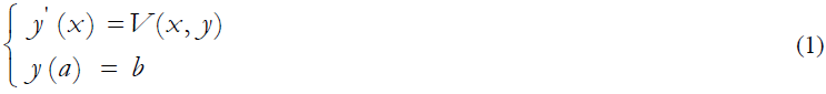
Sin utilizar gráfico alguno señala que, para un exiguo cambio h en la variable
independiente,  , podemos considerar que V(x,y) permanece
constante V(a,b)=A, concluyendo que la variable dependiente
, podemos considerar que V(x,y) permanece
constante V(a,b)=A, concluyendo que la variable dependiente  ,
experimentará una variación
,
experimentará una variación 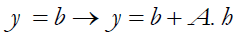 .
A fin de su construcción utiliza el concepto de infinitésimos, los cuales fueron
erradicados del análisis matemático [3].
.
A fin de su construcción utiliza el concepto de infinitésimos, los cuales fueron
erradicados del análisis matemático [3].
120
CADI 2014
Utilizando terminología actual y partiendo de la definición de derivada de Cauchy (1823) ensayamos una construcción equivalente.


Con los nuevos valores  construimos
  y repetimos
el proceso hasta llegar a los puntos distantes en el entorno que nos interesa, tal como
lo exhibe la siguiente tabla extraído del original de Euler.
y repetimos
el proceso hasta llegar a los puntos distantes en el entorno que nos interesa, tal como
lo exhibe la siguiente tabla extraído del original de Euler.
121
CADI 2014
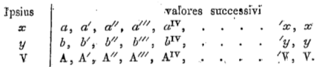
Fig.1 Tabla del original de Euler
La construcción matemática anterior genera el algoritmo exhibido, el cual está
destinado a ser ejecutado manualmente. Se propone su tratamiento por medios
computacionales. Las razones por obviar el uso de esta tecnología, se basan
principalmente en el hecho que puede interferir en el aprendizaje matemático y/o
reemplazar este por una tecnología que se torna obsoleta con rapidez asombrosa. Con
el debido cuidado en la selección de las herramientas computacionales, los principios
informáticos permanecen constantes, cambiando la interfaz con el usuario. Tras esta
interfaces actuales y considerando requerimientos del mercado, podemos hallar
programas escritos en los lenguajes más antiguos de computación como el LISP y
FORTRAN, en algunos casos traducidos al lenguaje C.
Continuando por el camino sugerido por el matemático Charles
122
CADI 2014
El anterior programa solo ejecuta de manera transparente un proceso rutinario. Los métodos numéricos comienzan tras la elaboración del algoritmo de Euler e independiente del medio en que este se ejecute.
Babbage y la
matemática Ada Lovelace, tenemos el siguiente programa para la ecuación diferencial
de primer grado  , con valor inicial
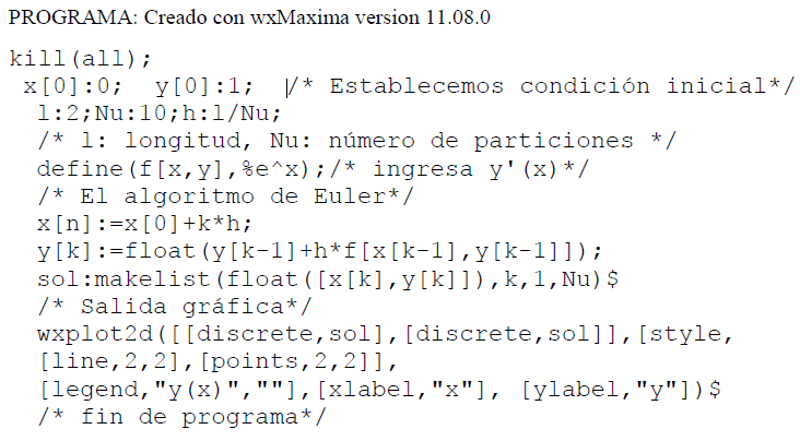
123
CADI 2014
La principal tarea matemática en métodos numéricos consiste en construir los conceptos cimentadores del llamado paradigma clásico: convergencia, estabilidad y consistencia [7].
La idea de convergencia está relacionada con el llamado error global, mientras que el concepto de estabilidad hace referencia a la manera en que los errores se propagan en el algoritmo.
La consistencia se relaciona con el llamado error local [8], estos conceptos son reportados como problemáticos [9]. En particular expondremos algunos tópicos sobre la construcción del concepto de consistencia, para ello definimos el “error local”, que es el error que se comete en un paso, partiendo del anterior considerado exacto.
En los métodos numéricos, siguiendo la línea de Euler, prosiguiendo con Runge, Heun, Kutta, Butcher y culminando en Dahlquist, podemos resaltar el carácter fundamental de los polinomios de Taylor. Estos son elementos con los que se construyen los métodos Runge-Kutta, dejando como herencia el orden de convergencia de estos al método numérico si ambos partiesen del mismo punto. En “Métodos Numéricos para Ingenieros” de Chapra[10] accedemos a un registro analítico y algebraico, donde emergen la familia de métodos
124
CADI 2014
Runge-Kutta2, en clara vinculación con los polinomios de Taylor.
A fin de reafirmar el concepto, recurrimos al software para generar gráficas en las que se observa que los polinomios de Taylor nos sirven de comparación, dentro de nuestros parámetros visuales, del grado de convergencia del método. (Fig. 2.)
125
CADI 2014
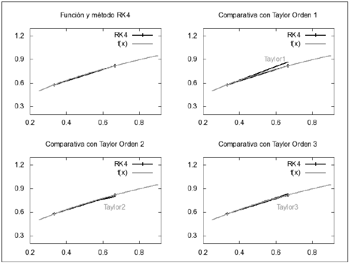
Fig.2 Polinomio de Taylor como regla para evaluar el orden de convergencia local.
126
CADI 2014
4 CONCLUSIONES
Podemos resumir nuestra investigación diciendo que matemática aporta para acotar y explicar los errores, determinar ámbitos de aplicación, mejorar algoritmos, interpretar resultados y supervisar la aplicación de las herramientas computacionales, siendo importante la integración de matemática e informática para la conceptualización de los métodos.
Cambiar el entrenamiento en resolver manualmente algoritmos, por el de volcarlos a un determinado sistema informático ayuda a la formación del pensamiento crítico.
La matemática que emerge como consecuencia del uso de los medios informáticos permite incursionar en los sistemas no lineales, de complicada resolución en forma analítica. La transparencia del proceso informático, la problemática de la transposición didáctica y el aprendizaje conceptual de los conceptos directrices, es la tarea fundamental del trabajo docente.
127
CADI 2014
REFERENCIAS
1. Artigue M.: Epistémologie et didactique. reserches en didactique des mathématiques. VOL.10, Nº 23(1990)- Epistemología y didáctica.
2. Euler (1768): De integratione aequationum differentialum, Cap. 7 De integratione aequationum differentialium per approximationem. Cálculo Integral. Volumen I).
3. Sanchez Ron J., Sanz Serna, J. Ildefonso Diaz, J., Bombal Gordón,F.: La obra de Euler. Tri-centenario del nacimiento de Leonhard Euler (1707-1783). Análisis Infinitesimal de Euler pag. 211.
4. Henrici, P., Discrete variable methods in ordinary differential equations, Wiley, New York 1962.
5. http://bibliotecadigital.ilce.edu.mx/sites/ciencia/volumen2/ciencia3/088/
html/sec_5.html.
6. Lady Ada Byron http://findingada.com/book/ada-lovelace-victorian-computing-vis.
128
CADI 2014
7. Sanz-Serna, J. M.: Stability and convergence in numerical analysis I: Linear problems-A simple, comprehensive account. En Nonlinear Differential Equations, Boston, 1985, 64–113; citado en Sanz Serna J.M.: Discurso leído en el acto de su recepción como Académico de Número por el Excmo. Sr. D. Jesús María Sanz Serna. Integración Geométrica (2007)
8. L. Héctor Juárez V. Análisis Numérico. Departamento de Matemáticas, Universidad Autó-noma Metropolitana
9. Caligaris M., Rodriguez, G. , Laugero, L.: La visualización en la compresión de errores que influyen en la solución numérica de un problema de valor inicial. III Jornadas de Enseñanza de Ingeniería. 2013. ISBN.2313-9056.
10. Chapra S., Canale R.: Métodos numéricos para ingenieros McGraw-Hill, 2007
129
CADI 2014
MÉTODOS DE VARIABLE COMPLEJA EN EL ESTUDIO DE LA DINÁMICA DEL FLUJO DE CALOR Descargar pdf
Alicia Tinnirello1, y Eduardo Gago1
1 Laboratorio Multidisciplinar de Ciencias Básicas,
Universidad Tecnológica Nacional,
Facultad Regional Rosario,
Zeballos 1341,
2000 Rosario, Argentina
Alicia Tinnirello, Eduardo Gago, egago@frro.utn.edu.ar
Resumen. Desde la línea de innovación educativa en Ingeniería se trabaja sobre nuevos paradigmas de enseñanza con la intención de lograr, un mayor desarrollo de capacidades intelectuales, adquisición de destrezas, sustitución de técnicas obsoletas por medios más eficientes y rápidos, y una mejor integración de conocimientos en el proceso de enseñanza aprendizaje. En función de esto, y con la inclusión de informática, hemos implementado la utilización de nuevas metodologías pedagógicas y diversas estrategias didácticas, apuntando al
131
CADI 2014
trabajo multidisciplinar en el desarrollo del tema Funciones de
variable compleja correspondiente a la asignatura Cálculo Avanzado en Ingeniería
Mecánica.
La propuesta didáctica que se presenta corresponde a un sistema relacionado
con la transferencia de calor en un fluido incompresible, donde los conceptos
del campo complejo y el flujo de fluidos son abordados analítica y gráficamente
dándole sentido a los contenidos curriculares, facilitando la interpretación y
conceptualización de la teoría.
Palabras Clave: Modelización, simulación, variable compleja, flujo de calor.
1 INTRODUCCIÓN
Los nuevos desafíos planteados en la Educación en Ingeniería, establecidos en los lineamientos de CONEAU para la acreditación de las carreras de grado; hacen necesaria una formación multidisciplinar del alumno, la cual se sustenta en la implementación de propuestas de aprendizaje que involucren
132
CADI 2014
la aplicación de los
recursos informáticos.
Las recomendaciones realizadas por los organismos de acreditación instan a que el
alumno desarrolle actividades de aprendizaje con herramienta computacional y
emigren del contexto de la clase magistral para proponer una estrategia metodológica
facilitada por el enfoque multidisciplinar. Se pretende que el alumno adquiera el
conocimiento mediante un proceso de experimentación, utilizando la simulación y la
visualización para ello debe plantear hipótesis de trabajo, inducir respuestas,
cuestionar predicciones y validarlas para darle significado a los aprendizajes.
Es posible resaltar un conjunto de contenidos mínimos indispensables, para la
formación básica del ingeniero que vienen siendo trabajadas en la Cátedra de Cálculo
Avanzado en la búsqueda de integrar las disciplinas en la carrera de Ingeniería
Mecánica, lo que implica por parte del docente el conocimiento de los programas de
enseñanza de las demás materias paralelas, no solo las del Tronco Integrador, sino de
materias básicas y de la especialidad, a fin de organizar dichas “prácticas
coordinadas” o de coordinar los problemas básicos de su materia con las situaciones
problemáticas que se
133
CADI 2014
desarrollan en Mecánica de Fluidos y Transferencia de Calor.
2 MOTIVACIÓN Y OBJETIVOS
El enfoque de la enseñanza multidisciplinar pretende relacionar los contenidos y los
conceptos impartidos en la clase con proyectos reales de ingeniería y de esta forma
dotar al futuro profesional de las herramientas necesarias para la detección de las
variables relevantes en un problema, interpretar y proponer soluciones ante diferentes
alternativas, aumentando su capacidad de análisis, la selección racional de propuestas,
y la toma de decisiones en base a las soluciones halladas.
Las actividades didácticas propuestas consisten en hacer énfasis en una investigación
teórica por parte de los alumnos con la tutoría de los profesores, para luego realizar
una analogía con los parámetros físicos del tema en estudio y por último con la
información reunida resolver la situación problemática propuesta con recursos
tecnológicos.
La propuesta metodológica de presentación de los contenidos matemáticos está
basada en la búsqueda de modelos que simulen la situación que se quiere formular o
la situación
134
CADI 2014
técnica en términos matemáticos, para lo cual se presenta una situación
simplificada, se traduce dicha situación en terminología matemática, y se trabaja con
dicho modelo. Esta metodología permite estimular el interés por el descubrimiento y
adquirir confianza en la utilización de los aspectos formativos de la Matemática,
relacionadas con otras áreas de conocimiento, como en este caso en el análisis de la
dinámica de un determinado fluido.
Los objetivos pedagógicos quedan planteados en las siguientes fases:
· Presentación de los sistemas a analizar
· Investigación teórica
· Modelización y análisis de los parámetros
· Interpretación de los resultados en términos técnicos
3 DESARROLLO DE LA EXPERIENCIA
Los sistemas que se analizan corresponden al flujo de calor en una región del plano complejo de un fluido incompresible en estado estacionario, no viscoso correspondiente a un campo irrotacional. En primer lugar se propone analizar el flujo de calor
135
CADI 2014
alrededor de un cilindro de sección transersal circular, y como segunda actividad se analiza el flujo de calor conocida la función de corriente.
3.1 Fundamentación teórica.
Se considera un medio conductor del calor con una distribución de temperatura que puede estar variando. La ley de Fourier de la conductividad del calor permite calcular la cantidad de calor conducido por unidad de área en una unidad de tiempo a través de un medio adecuado. Esta cantidad, se llama el flujo de calor a través de la medio circundante, y está dada por

En (1),  es el flujo de calor
  es el gradiente de temperatura complejo; y
  , es
una constante, que se denomina conductividad térmica y depende del material ó del
medio sobre el cual se está difundiendo.
Si
, es
una constante, que se denomina conductividad térmica y depende del material ó del
medio sobre el cual se está difundiendo.
Si  es una función de variable compleja unívoca en una región
  del plano
complejo
del plano
complejo  (tal que
  , donde
  es la unidad imaginaria), se
136
CADI 2014
dice
analítica en , si existe la derivada  en todo punto de .
La temperatura compleja está compuesta por el par ordenado cuya parte real es el
potencial de temperatura  y la parte imaginaria es la función de corriente
  .
.

Una condición necesaria para que sea analítica en una región , es que, y en
R , satisfacen las ecuaciones de Cauchy-Riemann
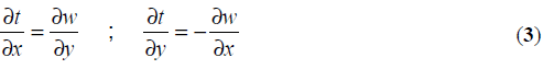
si estas derivadas parciales son continuas en , entonces las ecuaciones (3) son
condiciones suficientes para que sea analítica en . Las funciones que satisfacen
dichas condiciones se dicen conjugadas y armónicas.
Las funciones conjugadas y armónicas cumplen con las siguientes propiedades:
i) Propiedad de ortogonalidad, las curvas de las ecuaciones (4), son ortogonales
137
CADI 2014

ii) Si además las derivadas parciales segundas de y son continuas en , se
cumple la ecuación de Laplace
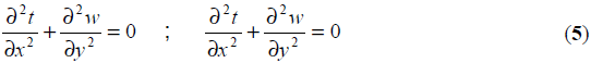
Si se limita el análisis del flujo de calor a un modelo de tipo bidimensional, entonces:
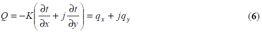
donde 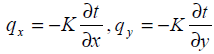 . Sea C una curva simple cerrada en el plano
complejo (que representa la sección transversal de un cilindro). Si
. Sea C una curva simple cerrada en el plano
complejo (que representa la sección transversal de un cilindro). Si  y
y  son las
componentes normal y tangencial del flujo de calor y si las condiciones de estado
estacionario se cumplen, de modo que no hay acumulación neta de calor dentro de
C , entonces se tiene:
son las
componentes normal y tangencial del flujo de calor y si las condiciones de estado
estacionario se cumplen, de modo que no hay acumulación neta de calor dentro de
C , entonces se tiene:

138
CADI 2014
Suponiendo que no hay fuentes o sumideros dentro de C . La ec. (6) resulta
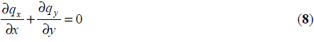
Lo cual llega a resultar que la componente es armónica 
Las ecs. (10) representan las líneas isotérmicas (o simplemente isotermas), y líneas de flujo de calor respectivamente.
3.2 Modelización, análisis y resultados.
1º Caso: Análisis del flujo de calor alrededor de un cilindro de sección transersal
circular
Se propone analizar el flujo de calor alrededor de un cilindro de paredes adiabáticas,
para una temperatura compleja cuya la ley
139
CADI 2014
es:
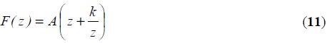
donde A es una constante positiva, y se considera la constante k > 0 .
Se plantearon los siguientes interrogantes:
a) ¿Qué relación existe entre el potencial de temperatura y la función de
corriente ?
b) ¿Cuáles son las ecuaciones de las isotermas y las líneas de flujo de calor?
c) ¿Cuál es la representación gráfica de las trayectorias anteriores? Interpretarlas
físicamente.
d) ¿Cómo es el perfil de temperaturas en los distintos puntos de su trayectoria?
e) ¿Cuáles son los puntos estacionarios?
f) ¿Cuál es la ecuación que mide la cantidad de calor en todos los puntos del
plano ?
g) Simular que sucedería si el flujo de calor dado
g1) el cilindro tuviera sección transversal elíptica
g2) no se enfrenta con el cilindro de paredes adiabáticas, y
140
CADI 2014
tuviera un sumidero
en el punto 
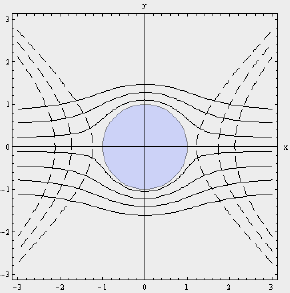
Fig.1 Curvas de flujo de calor e isotermas
Las funciones y , cumplen con las ecuaciones de Cauchy-Riemann, y
consecuentemente con la ecuación de Laplace, probando así que ambas funciones son
conjugadas y armónicas.
Las ecuaciones de las líneas de flujo de calor y las isotermas son, respectivamente:
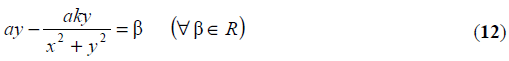
141
CADI 2014
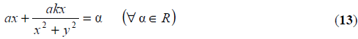
En la Fig. 1 se observó que las isotermas están marcadas con línea de puntos y son
ortogonales a las líneas de flujo de calor.
Las líneas de flujo de calor son paralelas al eje x, y se desvían al aproximarse al eje
y, rodeando al cilindro interpuesto en esa región. Estas curvas indican los caminos
que sigue el flujo de calor en dicha región del plano complejo . Cuando  corresponde a una trayectoria que se mueve en el eje x , o en el contorno de la
circunferencia de radio k .
corresponde a una trayectoria que se mueve en el eje x , o en el contorno de la
circunferencia de radio k .
La función que rige la cantidad de calor en el plano complejo :
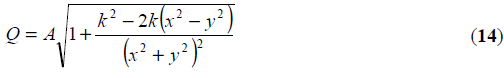
Se determino que si un observador situado en el origen se aleja del obstáculo la
cantidad de calor tiene su máximo valor  , es decir la cantidad de calor tiende a
un valor constante a medida que se aleja del obstáculo.
Los puntos estacionarios del sistema son aquellos donde la velocidad es cero y están
dados
, es decir la cantidad de calor tiende a
un valor constante a medida que se aleja del obstáculo.
Los puntos estacionarios del sistema son aquellos donde la velocidad es cero y están
dados
142
CADI 2014
por los valores de  y
y 
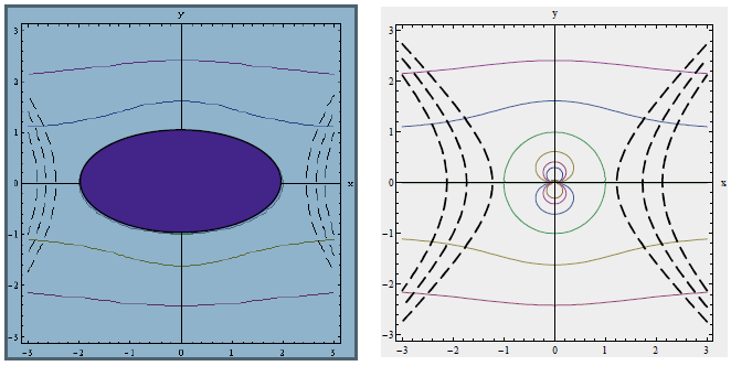
Fig.2 Curvas de flujo de calor e isotermas
En la Fig.2 se observó la simulación de situaciones alternativas a la dada originalmente. Se visualizó que cuando el flujo de calor se enfrenta con un cilindro de sección transversal elíptica, las líneas de flujo tienen una separación más amplia, mientras que las isotermas están más próximas. También, realizaron cambios en el sistema, la nueva simulación consistió en el suprimir el cilindro, y considerar un sumidero en el origen de
143
CADI 2014
coordenadas. Estos cambios modificaron el flujo de tal forma que se pudo observar que estando alejado del origen tenga el mismo comportamiento cómo si estuviera cualquier cilindro, pero en el origen de coordenadas el calor se disipa por el sumidero. 2º Caso. Análisis del flujo de calor conocida la función de corriente La función de corriente, en un sistema de transmisión de calor, es:
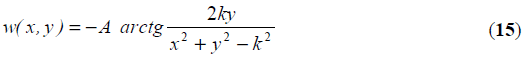
donde A es una constante positiva, y se considera la constante k > 0 .
Se plantearon los siguientes interrogantes:
a) ¿Cuál es el potencial de temperatura ?
b) ¿Cuáles son las ecuaciones de las isotermas y las líneas de flujo de calor?
c) ¿Cuál es la representación gráfica de las trayectorias anteriores? Interpretarlas
físicamente.
d) ¿Cómo es el perfil de temperaturas en los distintos puntos de su trayectoria?
e) ¿Cuáles son los puntos estacionarios?
144
CADI 2014
f) ¿Cuál es la ecuación que mide la cantidad de calor en todos los puntos del plano
?
El potencial de temperatura es:
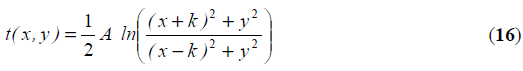
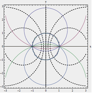
Fig.3 Curvas de flujo de calor e isotermas
En el flujo de calor que analizaron, la fuente de intensidad A situada en el plano
complejo en  , más el sumidero de intensidad -A situado en el plano
complejo en
, más el sumidero de intensidad -A situado en el plano
complejo en  . Las Ecs.
145
CADI 2014
(17), y (18) representan las ecuaciones de las líneas de flujo de calor y las isotermas, y son respectivamente:
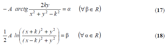
En la Fig. 3 se observaron que las líneas de flujo de calor son espirales logarítmicas
que se introducen en el origen, y las líneas de corriente son dos familias de
circunferencias ortogonales, y tienen similitud a las líneas de campo de un imán con
los polos situados en los puntos del plano complejo : y
4 CONCLUSIONES
El abordaje de actividades de carácter multidisciplinar desde las Ciencias Básicas, a través de la exploración de nuevos conocimientos, fomentan la creatividad a partir del análisis y el manejo de la información, lo que redunda en un proceso de
146
CADI 2014
enseñanza
aprendizaje innovador.
Para lograr la conceptualización teórica de los contenidos abstractos de variable
compleja fue fundamental poder analizar matemáticamente un sistema de transmisión
de calor, siendo la propuesta muy motivadora y el disparador de futuras
investigaciones., tales como la inquietud planteada por los propios alumnos de
completar el análisis con herramientas específicas para el tratamiento multifísico del
sistema.
REFERENCIAS
1. Cengel, J.; Cimbala, J.: Mecánica de Fluidos: Fundamentos y aplicaciones. México. 2ª
Edición. Editorial McGraw-Hill. México. (2006).
2. Bird, R., Stewart, W., Ligthfoot, E.: Fenómenos de Transporte, Reverté, México. (2011)
3. James, G.: Matemáticas Avanzadas para Ingeniería, Prentice Hall, 2ª Edición, (2002)
4. Tinnirello, A., Gago, E., Dádamo, M.: Designing Interdisciplinary
147
CADI 2014
Interactive Work: Basic Sciences in Engineering Education. The International Journal of Interdisciplinary Social Sciences. Vol. 5, fascículo 3, pp. 331-334. Cambridge. (2010).
148
EMCI 2015
GESTIÓN DEL CONOCIMIENTO MATEMÁTICO-COMPUTACIONAL: EXPLORACIONES PARA EL ABORDAJE DE LA COMPLEJIDAD Descargar pdf
Mónica Beatriz Dádamo, Alicia María Tinnirello
Laboratorio Informático Departamento Ciencias Básicas
Facultad Regional Rosario, Universidad Tecnológica Nacional
Zeballos 1341 (2000) Rosario, Argentina
mdadamo@frro.utn.edu.ar - atinnirello@frro.utn.edu.ar
Resumen. Este trabajo analiza las bases teóricas en la construcción de un conocimiento matemático-computacional propicio para el abordaje de la complejidad e independiente de la tecnología, en la enseñanza de matemática en las carreras de ingenierías no informática. Partiendo de un análisis histórico-epistemológico del desarrollo de la informática, sus puntos de contacto con la matemática tradicional y el impacto del computador en los procesos educativos, emerge la conexión entre las ciencias de la computación y la matemática, desarrollada por Alan Turing y Alonso Church, como canal
149
EMCI 2015
idóneo para la incorporación de fundamentos informáticos en la enseñanza de la matemática.
Palabras Clave: Máquina, Complejidad, Computacional, Autómatas, Modelado.
1 INTRODUCCIÓN
Existen múltiples formas de incorporar la informática en la enseñanza de matemática y asumimos que todas tienen razones valederas. El uso de instrumentos tecnológicos posibilita hacer más explícito el papel de los modos de representación. En particular, la manera en que la complementariedad entre lo gráfico, lo numérico, lo simbólico, lo algebraico y la simulación puesta de manifiesto en las experiencias realizadas, colaboraron a desarrollar los procesos de comprensión y la generalización y validación del conocimiento matemático.
Así, la incorporación de la computación a la matemática nos
150
EMCI 2015
conduce a un cambio en la gestión del conocimiento a través de una planificada experimentación, que muestra como algoritmos computacionales sugieren interesantes problemas matemáticos. Este campo es el de la matemática computacional, aquella cuyo objetivo es desarrollar algoritmos que permitan resolver problemas matemáticos tratados con el computador, particularmente aquellos problemas del dominio complejo donde emergen en forma natural lazos de realimentación como en los problemas de dinámica no-lineal. Siendo el computador el medio necesario para diversos desarrollos, existen formas habituales de utilizarlo, mediante un Sistema Algebraico Computacional (SAC), práctica más extendida en el ámbito universitario ingenieril, y/o mediante la programación en un determinado lenguaje o la programación en un SAC.
Los inconvenientes de mixturar el contenido matemático con el medio informático, más allá de las distintas epistemes que validan los conocimientos disciplinares, son: la rápida obsolescencia de los medios informáticos (caso del SAC DERIVE y del lenguaje BASIC) y las limitaciones propias del SAC o del lenguaje de programación.
151
EMCI 2015
En el caso de los SAC, si estos son cerrados y propietarios, carecemos de la posibilidad de acceder al conocimiento de sus algoritmos internos, sólo podemos entrenarnos en la interfaz de usuario [1]. En el caso de los lenguajes de computación, la elección es muy variada (creados más de 2500), con distintas potencialidades y limitaciones según su uso, regidos por diversos paradigmas destacamos el FORTRAN, presente en los SAC modernos aunque por dificultades en su aprendizaje y ejecución se los utiliza a través de una interfaz de usuario y el LISP desarrollado desde una perspectiva teórica matemático-computacional [2]. El uso mayoritario es en lenguaje C, C++ o los propios de los SAC.
Procurando elementos que permitan construir una base teórica sobre la cual sustentar el conocimiento matemático-computacional, compatible en tiempo y forma con la enseñanza universitaria y exenta de la problemática mencionada, se utiliza el concepto de Máquina de Turing. A través del mismo se posibilita la incorporación de ciertos contenidos de Matemática Discreta, aptos para el abordaje de la complejidad aun tratándose de carreras de ingenierías no informática, donde los contenidos curriculares de matemática
152
EMCI 2015
giran en torno a la Matemática del continuo [3].
2 CONSIDERACIONES HISTÓRICAS-EPISTEMOLÓGICAS DEL DESARROLLO DE LA COMPUTACIÓN
2.1 Antecedentes históricos
Si bien la introducción de dispositivos mecánicos para realizar cálculos es milenaria, como por ejemplo el ábaco, centramos la atención a partir de los trabajos de Charles Babbage y Ada Lovelace. Se trata del diseño de la máquina diferencial, la máquina analítica y la creación del primer programa computacional.Si bien la introducción de dispositivos mecánicos para realizar cálculos es milenaria, como por ejemplo el ábaco, centramos la atención a partir de los trabajos de Charles Babbage y Ada Lovelace. Se trata del diseño de la máquina diferencial, la máquina analítica y la creación del primer programa computacional.
Entre 1847 y 1849 Babbage se encaminó a diseñar la Máquina Analítica, basada en el mecanismo del telar que utilizaba tarjetas perforadas para controlar de manera automática el
153
EMCI 2015
diseño y los colores de los tejidos, diseñado por Joseph Marie Jacquard. Ésta resultaba más fácil de construir y tenía mayor poder de cálculo que la Máquina Diferencial, la cual había sido concebida en 1786 por Johann von Múller y usaba el sistema de numeración decimal. Así, diseña una computadora mecánica a la cual habrían de suministrarle datos e instrucciones a seguir a través de tarjetas perforadas de acuerdo con un código. La computadora a su vez proporcionaría las soluciones en forma de perforaciones en tarjeta. Como consecuencia, esta máquina "programable” ofrecía dos nuevas ventajas: i) por primera vez, una máquina sería capaz de utilizar durante un cálculo los resultados de otro anterior sin necesidad de reconfigurar la máquina, lo cual permitiría llevar a cabo cálculos iterativos, y ii) habría la posibilidad de que la computadora siguiese instrucciones alternas, dependiendo de los resultados de una etapa anterior del cálculo. Babbage describió esta máquina como "la máquina que se muerde la cola". Esta característica de "morderse la cola", describe la retroalimentación o realimentación, en el cual los datos de salida son retomados en la entrada [4]. Esta es una característica de los llamados sistemas complejos y en el
154
EMCI 2015
modelado matemático tradicional no se percibe. Las notas de Ada Lovelace sobre la máquina analítica de Babbage, son reconocidas hoy en día como el software de dicha máquina y la máquina analítica como modelo temprano del ordenador, motivo por el que Ada Lovelace es reconocida como el primer programador de la historia.
En el año 1920 el matemático David Hilbert presentó la exigencia de establecer la matemática sobre la base de un sistema axiomático completo y libre de contradicciones. Un sistema tal debe tener las características de Consistencia, Decibilidad y Completitud.
Un sistema tiene la propiedad de ser consistente cuando no es posible deducir una contradicción dentro del sistema, es decir, dado un lenguaje formal con un conjunto de axiomas, y un aparato deductivo (reglas de inferencia), no es posible llegar a una contradicción. Se dice de un sistema que es decidible cuando, para cualquier fórmula dada en el lenguaje del sistema, existe un método efectivo para determinar si esa fórmula pertenece o no al conjunto de las verdades del sistema. Cuando una fórmula no puede ser probada verdadera ni falsa, se dice que la fórmula es independiente, y que por lo tanto el
155
EMCI 2015
sistema es no decidible. La única manera de incorporar una fórmula independiente a las verdades del sistema es postulándola como axioma. Dos ejemplos muy importantes de fórmulas independientes son el axioma de elección en la teoría de conjuntos, y el quinto postulado de la geometría euclidiana.
Se habla de completitud en varios sentidos, pero quizás los dos más importantes sean los de completitud semántica y completitud sintáctica. Un sistema S en un lenguaje L es semánticamente completo cuando todas las verdades lógicas de L son teoremas de S. En cambio, un sistema S es sintácticamente completo si, para toda fórmula A del lenguaje del sistema, A es un teorema de S o no A es un teorema de S, esto es, existe una prueba para cada fórmula o para su negación En 1931 Kurt Gödel demostró que la coherencia y la completitud no podían ser ciertos a la vez en las matemáticas, o al menos en los números enteros. Por otra parte Alonso Church y Alan Turing demostraron que la matemática tampoco podía ser decidible, con lo que la idea de las matemáticas como sistema formal tal y como Hilbert pretendía, resultó dañada. El resultado de las acciones emergentes del Programa de Hilbert afectó concepciones de lo que la matemática es y lo que la
156
EMCI 2015
matemática no es. Nos centramos en el problema de la decibilidad, llamado Entscheidungsproblem.
Para resolver este problema Alan Turing ideo una máquina hipotética, hoy en día denominada Máquina de Turing, podemos concebir la naturaleza de esta máquina en forma dual: un objeto mecánico y un objeto matemático. De modo informal se puede decir que fue creada intelectualmente como un objeto matemático para leer una proposición matemática y dar un veredicto acerca de si esa afirmación es o no es demostrable, en un dado sistema. Hoy en día se toma como modelo general de una computadora.
En este programa propuesto por David Hilbert concurrieron entre otros, Kurt Gödel, Alonso Church, Stephen Kleene y Alan Turing todos ellos matemáticos de profesión y de diversas nacionalidades. La colaboración académica fue cortada durante la segunda guerra mundial y Alan Turing pasa a liderar la construcción de una máquina, destinada a descifrar los mensajes encriptados por la máquina alemana Enigma, lo cual es logrado, pero acontece bajo el secreto impuesto en el marco de una guerra a gran escala y prosigue luego en gran parte debido a las tensiones de la llamada guerra fría. De igual modo
157
EMCI 2015
y durante la segunda guerra mundial en EEU un grupo de científicos liderados por John von Neumann trabajaron en el desarrollo de computadores, también bajo estricto secreto militar.
2.2 Consideraciones paradigmáticas
Como se expresó anteriormente, existen diferentes formas de incorporar la informática en la enseñanza de la matemática, a fin de fundamentar la elección de modos y formas de incorporarla en la enseñanza, se considera conveniente responder y analizar las siguientes preguntas:
- ¿Consideramos a la computadora un artefacto tecnológico o una construcción matemática?
- ¿Consideramos a computadora un instrumento matemático, la esto es una máquina que podemos diseñar para que ejecute los algoritmos creados para resolver un determinado problema y ejecutar una dada simulación?
- ¿Incorporamos en la clase de matemática un determinado software matemático o un lenguaje de programación?
Si introducimos un software matemático específico, debemos
158
EMCI 2015
recordar que interactuamos con la interfaz de usuario, el problema matemático-computacional fue resuelto por quien elaboró el software y lo que realmente tenemos es un entrenamiento en el manejo de esa interfaz. Si el software es cerrado la matemática implicada queda cerrada, si el software es abierto y hay conocimiento del lenguaje de programación con que fue escrito, los algoritmos implicados se hacen visibles, del mismo modo que si trabajásemos programando en ese lenguaje. Sin embargo, sin conocer los límites teóricos y tecnológicos de la máquina, el conocimiento no será completo; conoceremos el cómo y no el porqué.
- ¿Utilizamos la computadora para hacer la misma matemática de siempre, más rápido y con menor esfuerzo o estamos lo suficientemente capacitados para llevar las matemáticas al nivel en que es capaz de generar algoritmos netamente computacionales?
Si continuamos con la matemática tradicional solamente, el problema consistiría en traducir los algoritmos manuales a un lenguaje de programación y esto sería todo, como de alguna manera se puede inferir.
En cierta medida, si aceptamos las soluciones pre-armadas de
159
EMCI 2015
las interfaces de uso general (Mathematica®, Matlab®, wxMaxima, Scilab®, etc.), sin un grado de conocimiento de las capacidades computacionales del ordenador, cuando éstos solucionan problemas que escapan al paradigma tradicional, será la tecnología quien los resuelva. Podremos enseñar a manipular esa tecnología para obtener la respuesta. Esa tecnología dejará de ser tal si conocemos la matemática que la hace posible.
- ¿Los algoritmos tienen la misma valoración y la misma significancia después de la introducción del ordenador?
Nuestra perspectiva es asignar a los algoritmos una importancia fundamental. Los algoritmos se convierten en el eje de la enseñanza considerando su adecuación a la realidad que se pretende modelar, su estabilidad, su robustez y las distintas formas en que estos pueden desarrollarse.
En el año 2002 asistimos a uno de los logros científicos más importantes de los últimos años, la descripción completa de la secuencia del genoma humano. Detrás de este logro se encuentra un algoritmo matemático que redujo drásticamente el tiempo necesario para completar la secuencia, y que fue principalmente desarrollado por el matemático Eugene Myers [5]. Podemos suponer que desde la misma matematización del
160
EMCI 2015
problema, se introduce en el modelo a formar tipos de solución que requieren algoritmos que serán ejecutados por máquinas [6, 7].
2.3 Reflexiones sobre las consideraciones
La contribución de la comunidad matemática al desarrollo de las ciencias de la computación es fundamental. Considerando que el modelo teórico actual del computador se desprende de la demostración de un teorema matemático, resulta cuasi-paradójica la temática como introducir el computador en la matemática, ya que éste es un producto de tal actividad. Esta conexión entre las computadoras y las matemáticas se utilizó más tarde para desarrollar las bases matemáticas para la ciencia informática. La pregunta: ¿Es posible utilizar la misma conexión para incorporar los fundamentos informáticos a la matemática-computacional?
Actualmente es posible construir el concepto de Máquina de Turing, partiendo del desarrollo de Autómatas Finitos (AF), siguiendo luego por el de Autómatas con Pila se llega a modelar con una Máquina de Turing, como se explícita en el
161
EMCI 2015
apartado 3.
Se disponen de herramientas informáticas gratuitas como el JFLAP (Java Formal Languages and Automata Package) en los cuales se puede probar y visualizar el comportamiento de lo antes mencionado [8]. Incluimos las funciones definidas en forma recursiva a fin de visualizar el tratamiento que tendrían las mismas en un autómata de pila.
Es decir, a partir de los pasos indicados, es posible comenzar a reconstruir la problemática de los algoritmos diseñados para ser ejecutados en ordenador.
3 DESARROLLO: CONEXIONES PARA LA INTERRELACIÓN COMPUTACIÓN-MATEMÁTICA
Según la Ordenanza 1027/2004 del Consejo Superior de la Universidad Tecnológica Nacional donde al prescribir distintos criterios metodológicos redacta “Las actividades deben ser seleccionadas en función de los problemas básicos de ingeniería y ser presentadas como situaciones problemáticas, que generan la necesidad de búsqueda de información y soluciones creativas” proponemos el siguiente problema o
162
EMCI 2015
meta-problema de Ingeniería Mecánica. En este caso en particular comenzamos con una pregunta fuertemente vinculada a la ingeniería: ¿Qué es una máquina?
Tratando de llegar a un concepto operativo respecto de la palabra máquina recurriremos a la matematización de este concepto, recordando las características clásicas de esta forma de proceder.
1. Presentarlo en forma abstracta, es decir independiente de su función, de los elementos que la componen, de la energía que utilizan, etc.
2. Debe ser tan general como se pueda. No interesan los casos particulares.
3. Debe admitir un tratamiento lógico-formal riguroso.
Comenzaremos con un ejemplo clásico que representa una máquina y a partir de ella observamos los elementos que conforman el modelo de Máquina de Estado Finito (FSM). El ejemplo concreto es una máquina expendedora de gaseosas [9] que entrega bebida gaseosa previo un pago que se realiza depositando monedas en la misma.
La máquina acepta monedas de $1.00 y $2.00. Cada lata cuesta $5.00 y si se deposita dinero de más lo retorna. Lo modelamos gráficamente en la Fig. 1.
163
EMCI 2015
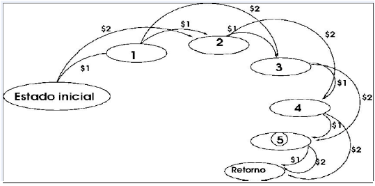
Fig.1 Modelo de máquina expendedora
La máquina parte de un estado inicial, que acepta monedas y de acuerdo a la moneda aceptada pasa a diversos estados: 1, 2, 3, 4, 5 y Retorno. El estado 5, se denomina estado de aceptación y desde ese estado se puede presionar el botón para que nos dé el refresco elegido y presiona este, retorna al estado inicial [9].
Ésta es la manera como en la teoría de la computación se describe a una máquina, en forma general hemos modelado un Autómata Finito Determinista. Autómata porque describe sistemas automáticos, finito porque el número de estados es finito y determinista porque para un dado estado y una dada
164
EMCI 2015
entrada solo hay una sola arista emergente. Tenemos a los Autómatas Finitos como un formalismo matemático para modelar todo tipo de máquinas, independiente de su construcción, finalidad, material, etc.
El poder expresivo de los autómatas finitos es poderoso. Incorporar esta forma de analizar las máquinas otorga una perspectiva distinta a la tradicional en las carreras de ingeniería y permite un interactuar más fluido en la incorporación de la informática o robótica a la ingeniería. La expendedora entregará la gaseosa solicitada si se cumplen previamente dos requisitos: Primero se depositaron monedas de $ 1.00 y $ 2.00, Segundo la combinación de esas monedas suma la cantidad exacta de $ 5.00. Ésta es la forma correcta de comunicarse con la máquina, el lenguaje que ella entiende.
¿Todo lenguaje puede ser reconocido por un autómata finito determinista? La importancia de esta pregunta es radical y no solo en ingeniería, tomando en cuenta que todas las máquinas construidas hasta la fecha se pueden modelar como autómatas finitos deterministas y que todo problema se puede plantear como el reconocimiento de cierto lenguaje, la pregunta y su respuesta equivale a decir: Dado un problema ¿Es posible
165
EMCI 2015
construir una máquina que los resuelva? La respuesta es NO. Por ejemplo, un AFD no puede reconocer lenguajes del tipo 0n 1n, es decir, secuencias tipo 01 0011 000111. Para profundizar en lenguajes regulares remitimos al libro de Jurado Málaga [10]. Ahora bien, existen otras máquinas teóricas denominadas autómatas de pila capaces de reconocer estos lenguajes, en particular el autómata finito de pila determinista (AFPD). Son similares a los autómatas finitos agregando a su estructura una pila que podemos comparar con una pila de platos, donde podemos poner o sacar los mismos de la parte superior, esto es, el último en ingresar será primero en salir. Las aristas del AFPD tienen etiquetas que indican de acuerdo con el símbolo de entrada y el plato que está en el tope de la pila, como reemplazar el plato.
Con el programa JFLAP podemos simular autómatas finitos, autómatas con pila y Máquinas de Turing, como se muestran en las Fig. 2, 3 y 4.
En la Fig. 3 se muestra el diagrama de estados de un AFPD que reconoce palabras del tipo 0n 1n.
166
EMCI 2015
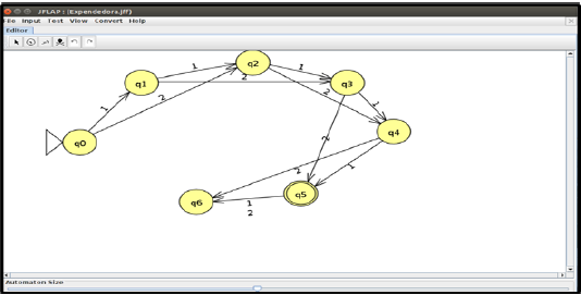
Fig.2 Autómata finito modelando la máquina expendedora de gaseosa
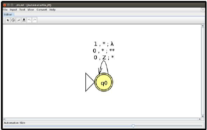
Fig.3 Autómata finito de pila determinista
167
EMCI 2015
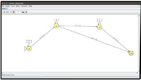
Fig.4 Sucesor de un número mediante la máquina de Turing
Estos pueden ser reconocidos por los llamados Autómatas de Pila. Sin embargo hay lenguajes que los
Autómatas de Pila no pueden reconocer, como el lenguaje que conste de cadenas de la forma ww donde w
pertenece a {0, 1}*. Algunas cadenas de este lenguaje son: 0001100011, 0101, 0000.
Lenguajes como éste solo pueden ser reconocidos por la Máquina de Turing, llamada así en honor al
matemático inglés Alan Turing. Siguiendo esta sencilla línea de los lenguajes con los que nos comunicamos a
los autómatas llegamos a la máquina de Turing.
168
EMCI 2015
3.1 Algunos ejemplos desarrollados en el laboratorio
El modelado de la máquina expendedora, utilizado como problema introductorio pasa a segundo plano,
quedando los autómatas como una perspectiva para interpretar o reinterpretar las máquinas que nos rodean y
lo utilizaremos para un segundo problema, introducir el computador como máquina matemática.
Para ello, mostraremos las funciones recursivas como la conexión entre la Máquina de Turing y las
matemáticas que fuera señalada en la tesis de Turing-Church.
Nos referimos a éstas como “funciones definidas en forma recursiva”, en lugar de la sintética y poco exacta
funciones recursivas.
En una primera aproximación esto sucede cuando en la definición de la función aparece la misma función,
sin embargo, a fin de no ingresar en un bucle infinito nos debe conducir hacia una interpretación más simple
de ella y que sea calculable, condición de parada.
Se presenta como ejemplo de función definida recursivamente la función factorial y la función exponencial.
Advertimos que el
169
EMCI 2015
foco está puesto en indagar el tratamiento que el computador da a los algoritmos. Función factorial:
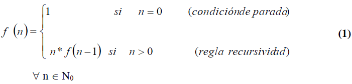
Habiendo expresado una función en forma recursiva mediante un algoritmo, profundizaremos el
conocimiento sobre este tema en la siguiente dirección:
¿Cómo se realiza esa tarea recursiva cuando se programa en un computador?
En la respuesta a esta pregunta recorreremos un camino que nos introduce a los fundamentos de la
Matemática Computacional y para ello utilizaremos los conceptos vertidos anteriormente. Comenzamos
revisando el concepto de pila.
Una pila es una estructura en la que se pueden añadir o eliminar elementos por un único extremo llamado
cima. Las eliminaciones se realizan en orden inverso a las inserciones. La pila en los autómatas vistos es
característica de los Autómatas
170
EMCI 2015
finitos con pila, deterministas y no deterministas. Una máquina de Turing puede simular un autómata de pila actuando sobre dos cintas. La primera cinta es la estándar de entrada, la segunda simula la pila. Asociaremos la pila a la memoria del computador y recordamos que la administración de la memoria y el tiempo forman parte de la problemática central de la computación real. Supongamos que al programa se le pide calcular el factorial de cuatro f (4), el primer paso será f (4) = 4*f (3), luego f (3) = 3*f (2) y así sucesivamente, como reflejamos en la siguiente tabla.
Tabla 1: La pila como recurso de algoritmo
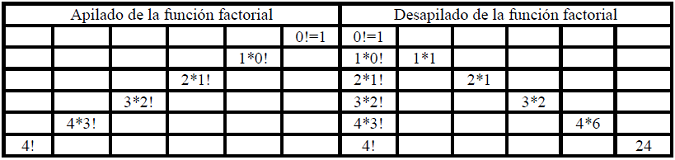
Disponemos de herramientas computacionales que hacen transparente esta forma de proceder en el ordenador, tal es el caso del lenguaje de programación LISP, el cual ejecutamos en
171
EMCI 2015
una interfaz gráfica del programa Máxima. Por medio del comando trace podemos visualizar el apilado y desapilado. Con el comando time tenemos el tiempo de ejecución. Algoritmo 1. Ejemplo del algoritmo recursivo de la función factorial escrito en Lisp, ejecutado en Maxima Algebra System sobre Linux.
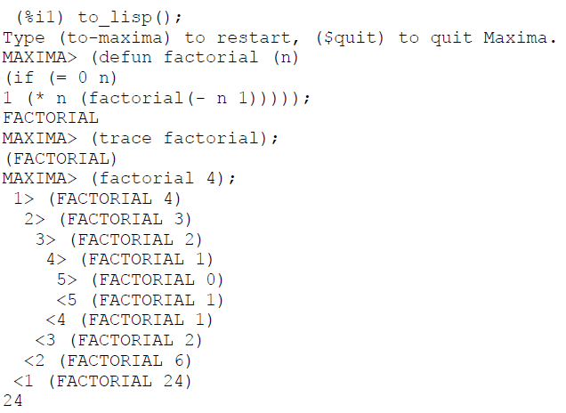
172
EMCI 2015
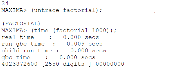
Cuando el algoritmo es diseñado para utilizar la estructura de pila acumula una sucesión de pasos hasta llegar al caso base, en ese punto regresa utilizando en cada paso la salida anterior de la función.
La segunda función es la exponencial que al estar definida en reales, no se amolda al tratamiento discreto propio del computador tradicional. En el tratamiento de la misma nos proponemos hacer visible el vínculo entre los autómatas finitos deterministas con pila y las funciones definidas en forma recursiva.
Emplearemos para aproximar esta función el Método de Euler para problemas de valor inicial (PVI), nuestro interés es revelar la estructura recursiva de este método y cómo un autómata
173
EMCI 2015
con pila lo resolvería. A los efectos de simplificar, omitimos la elaboración de un PVI y comentamos la capacidad del método de Euler de resolver sistemas complejos.
El modelado matemático de sistemas físicos se cristaliza en ecuaciones o sistemas de ecuaciones integro-diferenciales.
En casos más generales y simple el modelamiento conduce a ecuaciones de tipo y'(x)= f (x, y), que en la matemática tradicional nos lleva a una paradoja, ya que para conocer y(x) a partir de su derivada y'(x) esta toma como entrada el parámetro y, que es el que debo hallar. La forma de hallar solución a este tipo de problemas escapa a las elegantes soluciones tradicionales del cálculo. Quien incursionó sobre esta temática fue Leonard Euler (1707-1783), logrando el hoy denominado Método numérico de Euler, publicado en 1768.
Si una máquina resolviese esos algoritmos, tendría las características descriptas por Babbage: “la máquina que se muerde la cola”.
Nos interesa en particular un tipo de PVI, aquellos que se conoce una condición inicial y no se conoce la derivada en forma explícita, la cual depende de la función que pretendemos hallar. A diferencia de los PVI elementales, no podríamos
174
EMCI 2015
efectuar las gráficas de las derivadas antes de resolver el problema diferencial que admite una resolución aproximada siguiendo el método de Euler y es factible de ser ejecutado en una máquina tal como la proyectada por el matemático Charles Babbage y la matemática Ada Lovelace.
El hecho de discretizar nos permite que tome el resultado de una etapa anterior y se “realimente” de su salida, lo cual nos sitúa en la cibernética de primer orden. Tomamos la función exponencial ya que su derivada coincide con la función y podemos escribir situándonos a través de un ejemplo simple y conocido en el terreno de lo complejo. El hecho de aproximar no es lo sustancial del método de Euler y los siguientes [11, 12], de hecho la aproximación a través de la discretización en métodos como el Runge- Kutta4 (RK4), nos permite incursionar en el caos [13, 14]. Señalamos como sustancial en estos métodos, su capacidad de traspasar los límites del cálculo.
La rigurosidad de la matemática tradicional no se ve reflejada en este tipo de enfoque, porque lo que se busca es un sustento válido que permita pensar en las interacciones entre matemática y el computador.
Algoritmo 2. Ejemplo de la función exponencial f(x)= e0.5x,
175
EMCI 2015
f(0)=1, ejecutado en el programa wxMáxima.
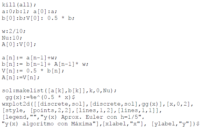
176
EMCI 2015
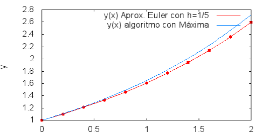
Fig.5 Aproximación de la función exponencial por el método de Euler
4 CONCLUSIONES
En una época como la actual, que se caracteriza por la escala, la incertidumbre y las nuevas dimensiones de la complejidad, muchos desafíos requieren soluciones que están fuera del alcance de un único pensamiento disciplinar [15].
Frente a los desafíos que debemos afrontar los docentes en la enseñanza de la Matemática en carreras de Ingenierías no informática, es necesario un cambio de perspectiva que nos
177
EMCI 2015
lleve a ver a la generación de algoritmos como actividad matemática por excelencia, y a la Informática, sustentada en gran parte por matemática discreta, como el conocimiento complementario para lograr su ejecución y gestionar sus salidas, las cuales reingresan al mundo físico matemático. Por ello, consideramos de suma importancia implementar estrategias áulicas que incorporen la relación matemática-informática para el abordaje de problemas del dominio complejo.
REFERENCIAS
1. Kay, A.: Programación de ordenadores. Investigación y Ciencia Nº 98/84. pp 15-23 (1984)
2. Graham, P.: Revenge of the Nerds. http://paulgraham.es/ensayos/la-venganza-de-los-nerds.html Accedido 1 de Julio de 2015
3. Carrera, E.; Canavelli, J.; Gaitán, M.: Actualizar el currículo de matemática. Una necesidad perentoria en Ingenierías. V Encuentro Nacional y II Latinoamericano La Universidad como objeto de
178
EMCI 2015
investigación (2007)
4. Instituto Latinoamericano de la Comunicación Educativa: La ciencia para todos. http://bibliotecadigital.ilce.edu.mx/sites/ciencia/volumen2/ciencia3/088/html/sec_5.html Accedido 2 de Julio de 2015
5. Martínez Dopico, F.: Matemática Computacional: Un nuevo pilar para el desarrollo científico y tecnológico en Matemáticas en la frontera: Nuevas infraestructuras matemáticas en la comunidad de Madrid. Ed. Comunidad de Madrid, Consejería de Educación, Dirección General de Universidades e Investigación. http://www.madrid.org/bvirtual/BVCM001757.pdf Accedido 29 de Junio de 2015
6. Wolfram S.: Programación en ciencias y en Matemáticas Investigaciones y Ciencias N° 98. pp 124-138 (1984)
7. Calegaris, M.; Rodriguez, G.: Simulaciones Computacionales: Autómatas Celulares. Primer congreso sobre Los Métodos numéricos en la enseñanza, la ingeniería y las ciencias- (EMNUS 2010)
179
EMCI 2015
8. www.jflap.org
9. Sagols Troncoso, F.: El arte de comprender el corazón de las máquinas. Cinvestav http://www.math.cinvestav.mx/sites/default/files/corazondelasmaquinas.pdf Accedido 1 de Julio de 2015
10. Jurado Málaga, E.: Teoría de autómatas y lenguajes formales. Ed. Universidad de Extremadura (2008)
11. Chapra, S.; Canale, R.: Métodos Numéricos para ingenieros. Mc Graw-Hill (2007)
12. J. M. Sanz-Serna: El método de Euler de integración numérica. http://sanzserna.org/pdf/37_eulerlibro.pdf Accedido 10 setiembre 2015
13. Dádamo, M.; Tinnirello, A.: Integración de conceptos en el análisis de los métodos numéricos: vinculación matemática-informática. Congreso Argentino de enseñanza en Ingeniería- (CADI 2014)
14. Gaylord, R.; Wellin, P.: Computer Simulations with Mathematica. Telos-Springer Verlag. (1995)
180
EMCI 2015
15. Van Der Linde, G.: ¿Por qué es importante la interdisciplinariedad en la educación superior? Cuaderno de pedagogía Universitaria, Año 4. N°8: 11-13. (2007).
181
EMCI 2015
ANÁLISIS DINÁMICO PARA LA MODELIZACIÓN DE SISTEMAS CON FUNCIONES COMPLEJAS Descargar pdf
Alicia M. Tinnirello, Eduardo A. Gago
Laboratorio Informático y Multidisplinar de Ciencias Básicas,
Universidad Tecnológica Nacional, Facultad Regional Rosario
Zeballos 1341
{atinnirello, egago}@frro.utn.edu.ar
Resumen. En este trabajo se presenta un diseño metodológico implementado en la enseñanza de la asignatura Cálculo Avanzado en la carrera Ingeniería Mecánica para el desarrollo de Funciones de variable compleja, teniendo en cuenta la importancia de gestionar el conocimiento matemático mediante la utilización de sistemas de cálculo computacionales. Se analiza un sistema dinámico con un fluido perfecto, es decir con el movimiento de un fluido incompresible, donde los conceptos del potencial complejo y el flujo de fluidos son abordados analítica y gráficamente dándole sentido a los contenidos curriculares, facilitando la interpretación y conceptualización. Esta
183
EMCI 2015
metodología de trabajo habilita la enseñanza de matemática centrada en el análisis dinámico que describe el comportamiento de un sistema y la visualización de los resultados, favoreciendo el abordaje multidisciplinar desde las Ciencias Básicas.
Palabras Clave: Modelización, Simulación, Variable compleja, Flujo de fluidos.
1 INTRODUCCIÓN
Los avances en la informática y la comunicación han provocado la génesis de un nuevo paradigma en la enseñanza de las ciencias básicas, optimizando el desarrollo de las capacidades intelectuales de los estudiantes mediante la adquisición de un conjunto de habilidades que permiten organizar, representar y codificar la realidad, sustituyendo los sistemas de enseñanza tradicional.
Es importante que el estudiante aplique el conocimiento básico en diferentes campos mediante la resolución de modelos cada
184
EMCI 2015
vez más complejos que requieren el uso de software específicos, evidenciando la conexión de conceptos en ciencias básicas, con las herramientas necesarias para el modelado y la simulación en problemas de ingeniería [1].
Una nueva definición del perfil profesional está basada en las competencias que desarrolla el estudiante en el transcurso de su carrera universitaria, situación fuertemente influenciada por las incumbencias requeridas por los organismos responsables de acreditación de los programas de ingeniería que proponen continuas innovaciones [2].
Con el objetivo de llevar adelante estos cambios necesitamos adecuar la currícula universitaria no sólo a nuevas metodologías de trabajo que permitan la estimulación del desarrollo intelectual, sino también que tengan un enfoque multidisciplinar. El objetivo no es enseñar y aprender solamente matemáticas, sino hacerlo enfrentándose con casos reales y sistemas sencillos que conduzcan al alumno a tener una mirada sobre la relación entre las disciplinas que componen su formación profesional.
Para lograr que el proceso de enseñanza sea eficaz, es importante diseñar actividades curriculares basadas en el
185
EMCI 2015
aprendizaje por construcción de conceptos, donde se persiga como objetivo tener un alumno desarrollándose en plena actividad, que sea protagonista del proceso de enseñanza aprendizaje, y hacer énfasis en el carácter inter y multidisciplinario inherente a las carreras de Ingeniería. La selección de modelos matemáticos alternativos influye favorablemente en el interés por parte de los estudiantes, y si la propuesta de trabajo resulta atractiva y conveniente entonces se logra analizar y visualizar sistemas complejos para una mejor apropiación del tema en estudio.
2 OBJETIVOS
Se implementa un sistema de aprendizaje de Matemática donde se visualicen los conceptos relativos a las funciones de variable compleja, como ceros, polos y sus órdenes de multiplicidad, singularidades, etc., a través de una herramienta computacional que por su interactividad y versatilidad permite comprender la topología de los puntos que se quieren analizar en diferentes sistemas físicos. Así también generar nuevos estilos de trabajo para cambiar el modelo
186
EMCI 2015
teoría-práctica-aplicaciones y lograr espacios de aprendizaje que habiliten el uso de información numérica y simbólica durante el desarrollo de los temas y reforzar la conceptualización mediante diseños gráficos cuya complejidad requiere de habilidades y capacidad de análisis.
Se pretende que la interacción entre las distintas áreas del conocimiento permita potenciar la capacidad de los estudiantes en la adquisición de conceptos para su consiguiente utilización en los modelos requeridos para la resolución de problemas ingenieriles.
3 METODOLOGÍA
La problemática de fondo de como impartir la enseñanza reside en crear las condiciones para que los esquemas de conocimiento que construye el alumno evolucionen en un sentido determinado. La cuestión clave no reside en si el aprendizaje debe conceder prioridad a los contenidos o a los procesos, sino en asegurarse de que sean significativos y funcionales.
El alumno necesita disponer de conocimientos previos
187
EMCI 2015
suficientes a partir de los cuáles poder abordar los modelos propuestos, con el fin de establecer relaciones entre ellos lo más complejas y ricas posibles que le permitan aumentar el significado de sus aprendizajes [2].
Es conveniente ayudar en primera instancia al alumno a reordenar y asimilar los conceptos teóricos necesarios, para que pueda abordar satisfactoriamente los aprendizajes programados, y de esta forma se elaborarán las estrategias adecuadas para propiciar situaciones favorables de aprendizaje.
El diseño de actividades curriculares basadas en el análisis dinámico de sistemas físicos que involucren un aprendizaje por construcción de conceptos, fomenta el interés por parte del alumno para su participación como sujeto activo del proceso de enseñanza aprendizaje, y se aproxima al carácter multidisciplinario que debe darse en el desarrollo de los planes de estudio en carreras de Ingeniería [1-2].
Las actividades didácticas propuestas consisten en hacer énfasis en una investigación por parte de los estudiantes siempre con la asistencia de los profesores, con la intención de realizar un análisis pormenorizado de los parámetros físicos del tema en estudio y encontrar la relación respecto a los
188
EMCI 2015
conceptos teóricos desarrollados lo que redunda en la conceptualización del tema.
4 SISTEMA DE ESTUDIO: FLUJO DE FLUÍDOS
Las actividades que se describen están orientadas hacia los alumnos de la asignatura Cálculo Avanzado de la carrera Ingeniería Mecánica, y toman como premisa los conocimientos básicos del tema Funciones analíticas de Variable compleja.
Los alumnos desarrollan la experiencia en el Laboratorio Informático y Multidisciplinar de Ciencias Básicas y utilizan como herramienta computacional el software WOLFRAM MATHEMATICA, en su versión 8.0. MATHEMATICA es uno de los programas de matemática más completos para realizar cálculo simbólico, numérico y gráfico; con una cantidad considerable de funciones integradas, y con aplicaciones a distintas disciplinas.
La propuesta que se presenta se puede realizar gracias a las posibilidades tecnológicas de representación y cálculo con las que se cuentan en la actualidad, ya que en un pasado no muy lejano, muchos casos relativos a la Variable compleja eran
189
EMCI 2015
imposibles de analizar, no sólo en forma analítica sino también gráficamente.
Muchos problemas importantes de flujo de fluidos se resuelven, en forma no excluyente, analíticamente mediante métodos de variable compleja. El sistema que se analiza corresponde al flujo bidimensional de un fluido incompresible, no viscoso correspondiente a un campo irrotacional que se mueve en estado estacionario con velocidad constante para distintos valores del potencial complejo de velocidad. Es decir, las componentes de la velocidad se obtienen mediante la derivación de una función potencial llamada potencial complejo que se trata de modelizar y cuya caracterización debe establecerse con los conceptos teóricos desarrollados [3-5].
4.1 1ª Sesión: Investigación del marco teórico del tema
Para analizar el sistema los alumnos realizan las suposiciones sobre el flujo de fluidos que les serán de utilidad para estudiar y modelizar un flujo ideal, es decir:
El flujo del fluido es bidimensional: Es un modelo de flujo básico y las características del movimiento del fluido se estudian en un
190
EMCI 2015
plano, son esencialmente las mismas en todo plano paralelo. Lo que permite confinar el estudio del fluido a un plano simple, el cual se desarrolla en el plano complejo z. Las figuras construidas en este plano se interpretan como secciones transversales de cilindros infinitos perpendiculares al plano.
El flujo es estacionario o uniforme: La velocidad del fluido en un punto depende de la posición y no del tiempo.
Las componentes de la velocidad derivan de una función potencial.
El fluido es incompresible: El fluido tiene densidad constante.
El fluido es no viscoso: El fluido no tiene viscosidad o no tiene fricción interna. Si no hay viscosidad, las fuerzas de presión sobre la superficie son perpendiculares a dicha superficie.
Con las consideraciones realizadas se desarrolla la propuesta dando el significado físico a las funciones utilizadas y su derivada, conectando conceptos e investigando comportamientos [3-5].
4.2 2ª Sesión: Modelización del sistema en estudio
La resolución del modelo matemático que responde al sistema
191
EMCI 2015
físico requiere de un trabajo autogestionado de los alumnos. Con este propósito, se formaron dentro del curso comisiones de tres alumnos cada una, que con el material bibliográfico sugerido y el asesoramiento de los docentes se llegó a obtener conclusiones teóricas de los conceptos a utilizar en la propuesta de trabajo, de acuerdo a nuestra solicitud, luego de escuchar y revisar las conclusiones a que llegó cada grupo se hizo un debate sobre el tema proponiendo el siguiente marco teórico:
El potencial de velocidad complejo F es una función analítica de variable compleja unívoca en alguna región R del plano z está compuesta por el par ordenado cuya parte real es el potencial de velocidad  y la parte imaginaria es la función de corriente
  [6-7].

siendo jla unidad imaginaria
Se dice que F es analítica en dicha región R si existe la derivada F' en todo punto z de dicha región R.
La velocidad de circulación de un fluido 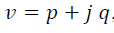 es el gradiente del potencial
192
EMCI 2015
de velocidad

De las ecuaciones (1) y (2) se pudo expresar la velocidad del fluido con la ecuación (3)

Derivando el potencial complejo a partir de la ecuación (1) se obtuvo la ecuación (4)

Una condición necesaria para que F sea una función analítica en una región R, es que en R, y cumplan las condiciones expresadas por las ecuaciones de Cauchy-Riemann:
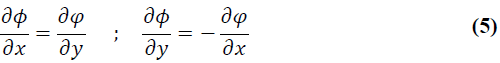
Si las derivadas parciales en la ecuación (5) son continuas en R, entonces las ecuaciones de Cauchy-Riemann son condiciones suficientes para que F sea analítica en R.
193
EMCI 2015
La familia de curvas de ecuaciones:
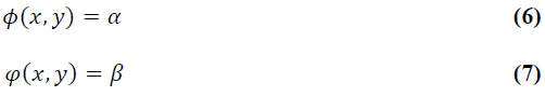
donde  y
y  son constantes, son ortogonales y las ecuaciones (6) y (7) se denominan ecuaciones de las curvas equipotenciales y ecuaciones de las líneas de corriente, respectivamente. En el movimiento uniforme, las trayectorias representan los caminos reales de las partículas del fluido en el modelo de flujo.
Con el modelo logrado y mediante las ecuaciones (4) y (5) se pudo deducir que la velocidad del fluido es el complejo conjugado, derivada de la función F.

Se observa que las imágenes de la función expresada en la ecuación (8) son números complejos y conjugados, de manera tal que es posible expresarla por medio de la ecuación (9)

194
EMCI 2015
Para poder calcular el módulo de la velocidad del fluido |v| se utiliza la ecuación (10)

Además, si F es analítica, entonces sus componentes y son funciones armónicas en R2. Una función se dice armónica en R2 si se satisface la ecuación de Laplace. En las ecuaciones (11) y (12) se enuncian las expresiones de la Ecuación de Laplace que deben satisfacer y .
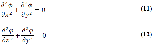
4.3 3ª Sesión: Análisis del potencial de velocidad complejo
Se suministra como dato el Potencial de velocidad complejo F, cuya ley es:
195
EMCI 2015
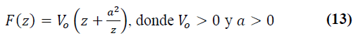
A partir del Potencial complejo F expresado en la ecuación (13), y de acuerdo a la modelización del sistema contemplada en el ítem 4.2, se propone a los alumnos que diseñen a modo de guía, una batería de actividades y consignas que les permitan estudiar dicho Potencial complejo con el objetivo de arribar a conclusiones significativas del modelo planteado [5].
Algunas de las consideraciones que los alumnos estimaron necesario investigar, fueron las que se detallan a continuación:
Ceros y polos.
- Líneas de corriente y líneas equipotenciales.
Análisis del perfil de velocidades del fluido en los distintos puntos de su trayectoria.
Puntos estacionarios.
Régimen del fluido
Puntos de singularidad
Interpretación física de los parámetros estudiados.
Los alumnos eligen arbitrariamente en la ecuación (13) un valor unitario de los valores de las constantesV0 y a, para poder
196
EMCI 2015
realizar las representaciones gráficas en el plano y en el espacio asociadas a F, con el propósito de interpretar sus características.
Todas las actividades se desarrollan en el Laboratorio Informático y Multidisciplinar de Ciencias Básicas con la asistencia del cuerpo docente, y se trabaja con las computadoras que se tienen disponibles, y además algunos alumnos, por su comodidad, traen sus computadoras personales.
En el desarrollo de la clase, todos los alumnos trabajan con el programa MATHEMATICA, ya que con dicho programa se realizan los trabajos prácticos de Cálculo Avanzado, y también se han realizado los trabajos prácticos de Laboratorio en primero y segundo año en las asignaturas del área Matemática y en Fundamentos de Informática.
En primera instancia los alumnos con el dato de la ley del Potencial complejo F discriminan la parte real y la parte imaginaria de dicha función, expresión que se enuncia en la ecuación (14) y por medio de ella pueden realizar la gráfica de la Fig. 1.
197
EMCI 2015
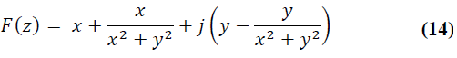
En la Fig. 1, los alumnos observan que las líneas de corriente son las curvas que indican el recorrido que siguen las partículas de fluido y tienen una trayectoria paralela al eje x. Además concluyen que cuando la función de corriente resulta nula  , se evidencian dos posibilidades bien diferenciadas: en puntos alejados del origen, la trayectoria del fluido se mueve en una dirección coincidente con el eje x; mientras que a medida que se produce un acercamiento a las proximidades del obstáculo el movimiento de las partículas del fluido se orientan alrededor del contorno de la circunferencia de radio unitario.
198
EMCI 2015
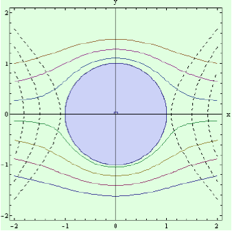
Fig.1 Líneas de corriente y curvas equipotenciales de F.
Se citan a continuación el resto de las conclusiones a las que arribaron los alumnos respecto a su trabajo con el Potencial complejo F:
Las líneas equipotenciales están marcadas con línea de puntos y son ortogonales a las líneas de corriente, que están dibujadas con curvas de trazo continuo. Además para este caso observaron que todas las curvas equipotenciales particulares asociadas a la ecuación (13), son asintóticas a las rectas
199
EMCI 2015
de ecuaciones:

La circunferencia de radio unitario representa una trayectoria y como no puede haber flujo a través de una trayectoria, se puede considerar como un obstáculo circular de radio unitario que está situado en el camino del fluido.
El módulo de la velocidad compleja posee un valor variable cerca del obstáculo y su expresión es:
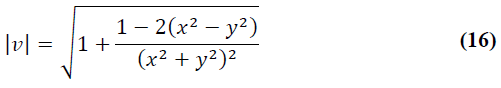
En este caso, observaron que a medida que se analizan puntos que se alejan del obstáculo la velocidad asume el valor unitario, y se concluye que el fluido está transitando su recorrido en la dirección del semieje positivo 𝑥 con velocidad constante de valor unitario.
La Fig. 2 permite observar en forma conjunta los ceros y los polos de F, los alumnos determinan en base a dicha gráfica que los ceros que posee el Potencial complejo F se encuentran en
200
EMCI 2015
los puntos del plano complejo z de coordenadas:  y
y 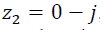 , mientras que para F el único polo simple que posee se localiza en
un punto el plano complejo de coordenadas:
, mientras que para F el único polo simple que posee se localiza en
un punto el plano complejo de coordenadas: 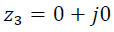 .
.
Además concluyeron que el centro del obstáculo de sección plana circular coincide con las coordenadas del
polo en F. Entonces si no estuviera el obstáculo, el fluido desaparecería. Dicho punto que presenta esta
característica se denomina sumidero de F.
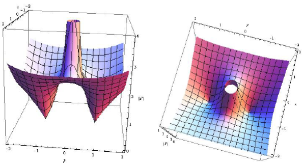
Fig.2 Ceros y polos de F.
201
EMCI 2015
En la Fig. 3 observaron una vista en el espacio con mucha precisión del único polo simple de F. El polo se destaca dentro de la gráfica por ser un pico de altura considerable.
Fig.3 Polos de F.
En la Fig. 4 se visualizan las gráficas de las curvas de nivel de las superficies mostradas en la Fig. 2 y 3, la región que aparece en color blanco indica la existencia del polo, y las zonas más oscuras revelan la posición de los ceros de F.
202
EMCI 2015
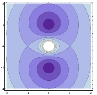
Fig.4 Curvas de nivel para identificar el polo de F.
Los alumnos indagan y verifican además, que hay una condición matemática que relaciona directamente la
existencia de un polo con la velocidad del fluido. Dicha condición se enuncia en la ecuación (17), y se cumple
cuando existe un polo simple para sistemas físicos cuyos Potenciales de flujo son del tipo como el que fue
propuesto en la ecuación (13).
En esta instancia, se puede afirmar que los alumnos no sólo aplican los conceptos inherentes al tema de la
Variable Compleja al estudio de la trayectoria de los fluidos, sino que
203
EMCI 2015
además necesitan conocer contenidos de la asignatura tales como: Límite de Funciones complejas.
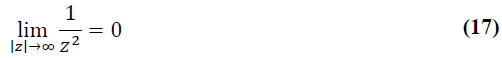
Si se cumple la ecuación (17), entonces se puede verificar la condición física del fluido establecida. El
sentido de ese límite corresponde a que físicamente que la velocidad del fluido se mantiene constante más allá
del obstáculo.
En la gráfica de la Fig. 5 observaron únicamente los ceros del potencial complejo F. Dicha gráfica tiene la
particularidad de destacar los ceros mediante la visualización de dos picos en la zona inferior de la gráfica de
la superficie.
204
EMCI 2015
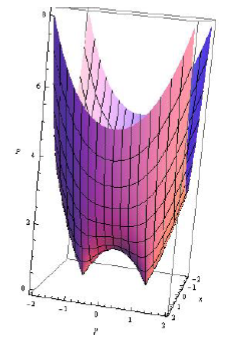
Fig.5 Ceros de F.
Las curvas de nivel de la gráfica de la Fig. 6, muestran que el polo y los ceros están en la zona más opaca de la figura. El polo es el punto de intersección entre los dos lóbulos oscuros, y los puntos medios de cada uno de los mismos ubican a los ceros de F.
205
EMCI 2015
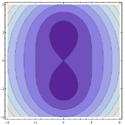
Fig.6 Curvas de nivel para identificar los ceros de F.
Los puntos estacionarios del sistema son aquellos donde la velocidad es cero, y corresponden a los ceros de
la Función velocidad que es la derivada de la función F y se encuentran en los puntos de la Fig. 7 dados por
los puntos del plano complejo de coordenadas de 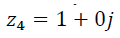 y
y 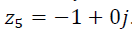 .
.
206
EMCI 2015
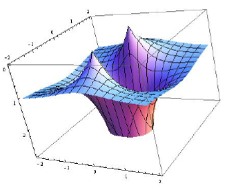
Fig.7 Puntos estacionarios de F.
5 CONCLUSIONES Y TRABAJOS FUTUROS
Es interesante destacar como el uso de funciones de variable compleja ha permitido el estudio de sistemas físicos hipotéticos dándole sentido a los aprendizajes y permitiendo que el proceso de enseñanza involucre varias disciplinas favoreciendo la comprensión y fomentando el interés por la Matemática y sus desarrollos.
La importancia de trabajar con diversas fuentes documentales, problemas, guía de estudio, libro de texto, bibliografía asociada,
207
EMCI 2015
simulaciones virtuales y fomentar la capacidad de autogestión en los procesos de aprendizaje ha desarrollado el interés para relacionar los conceptos y lograr el enfoque multidisciplinar en la gestión del conocimiento matemático-computacional.
Es importante señalar que las visualizaciones realizadas en el desarrollo de la clase con el apoyo de herramientas computacionales colaboraron para que el fundamento de los temas involucrados en Funciones de variable compleja pierda la cuota de abstracción y generalización que suele asociarse al aprendizaje de estos conceptos. Además, el ambiente colaborativo desarrollado en el Laboratorio de Ciencias Básicas fue propicio para poner en valor actividades de investigación que permitan al estudiante inferir lo próximo y autogestionar su propio conocimiento.
Los trabajos futuros tratarán sobre la dinámica de fluidos computacional y su introducción en los proyectos a desarrollar con alumnos del tercer nivel de la carrera de Ingeniería Mecánica.
208
EMCI 2015
REFERENCIAS
1. Tinnirello, A.; Gago, E.; Dádamo, M.: Integración multidisciplinar: Matemática computacional -Mecánica de fluidos. Trabajos III CAIM -2012. Tercer Congreso Argentino de Ingeniería Mecánica. pp. 430-441. (2012)
2. Tinnirello, A.; Gago, E.; Dádamo, M.: Designing Interdisciplinary Interactive Work: Basic Sciences in Engineering Education. The International Journal of Interdisciplinary Social Sciences; Publisher Site: http://www.SocialSciences-Journal.com; Vol. 5, Nº 3, pp. 331-334. (2010)
3. Bird, R; Stewart, W.; Ligthfoot, E.: Distribuciones de velocidad con más de una variable independiente: Fenómenos de Transporte; Editorial Limusa Wiley; pp. 141-150 (2012)
4. Mott, R.: La naturaleza de los fluidos y el estudio de su mecánica: Mecánica de Fluidos; Editorial Prentice Hall; pp. 10-51 (2006)
5. Cengel, J.; Cimbala, J.: Mecánica de Fluidos: Fundamentos y aplicaciones; Editorial McGraw-Hill. pp. 136-158. (2006).
209
EMCI 2015
6. James, G.: Funciones de una variable compleja: Matemáticas Avanzadas para Ingeniería; Editorial Prentice Hall; pp. 28-41 (2002).
7. Churchill, R.; Brown, J.: Funciones analíticas: Variable compleja y aplicaciones; Editorial Mc Graw Hill; pp. 49-71 (2004)
210
ICERI 2015
DESIGN AND SIMULATION OF MECHANICAL EQUIPMENT BY DESIGN TOOLS AND MULTIPHYSICS PLATFORMS Descargar pdf
Alicia Tinnirello1,2, Eduardo Gago1, Mariano Valentini1
1 Universidad Tecnológica Nacional Facultad Regional Rosario (ARGENTINA)
2 Universidad Nacional de Rosario Facultad de Arquitectura, Planeamiento y Diseño
(ARGENTINA)
Abstract. New challenges in engineering teaching require a multidisciplinary training of future engineers through the incorporation of computer resources that enable the modeling, simulation and design of real physical systems. The teaching methodology that provides to these new requirements, should consider the implementation of modelling and simulation tools, to offer a form of updated engineering work and according to technological advancement. The approach of multidisciplinary teaching in engineering careers should relate the contents and concepts taught in class with real projects in the engineering
211
ICERI 2015
field, with the purpose of enriching the training of the professional future, through the use
of tools for the detection of the relevant variables in a problem, interpret, and propose solutions to
different alternatives increasing their capacity for analysis, and above all for the rational selection of
proposals, and taking decisions based on the solutions found.
The proposal presented aims to show a work in an integrated manner using Design CAD (Computer
Aided Design) and a multiphysics software simulation, CFD (Computer Fluid Dynamics), with the
purpose to study the fluid dynamics of an equipment, in this case the distribution of flow velocity
patterns in tube condensers, to analyze the erosion-corrosion mechanism in tubes to eliminate faults
by modifications on design.
The advantages of working with simulation platforms replaced the work of analytical resolution, where
the amount of variables involved makes very complex analysis. This methodological proposal
suggests an important breakthrough in process engineering, since is used the development of
simulation tools for product design through platforms that incorporate calculation by finite element and
computational fluid dynamics.
To simulate the operation of equipment, in order to obtain
212
ICERI 2015
the desired performance optimization.
COMSOL Multiphysics platform allows us to import models from designs of solids such as SOLID
WORKS programs. This interaction between programs is very useful for the design of complex
geometries. The designed models for different air intakes are analyzed taking into account that the
assumptions about the behavior of the density changes of pressure and/or temperature are very
important in the study of flows. Application to fluid module is intended for incompressible, however
admits small changes in density caused by temperature variations. They are presented in 3D, in the
final work, different models designed for different velocities, and flux flow variations and the analysis of
the mass flow rate input that defines the choice of the appropriate design.
Keywords: CAD; Simulation; CFD technology; Fluid flow; CAD.
1 INTRODUCTION
The new challenges in Engineering Education, require a
213
ICERI 2015
multidisciplinary training of future engineers
by incorporating computing resources to the modeling and simulation of real physical systems.
To achieve the approach of the multidisciplinary learning in engineering careers it is necessary to link
the content and the concepts taught in the class with real projects in the engineering field with the
purpose to enrich the training of future professional with the necessary tools for the detection of the
relevant variables in a problem, interpret, and propose solutions to different alternatives, increasing its
capacity for analysis, the rational selection of proposals, and the decision-making on the basis of
solutions found.
Even more, emphasis should be placed in that the engineer can interact with several design and
simulation tools, pondering its versatility. This form of work, and the implementation of modeling tools, allows engineers to give you a great scope to his research and incorporate a form of engineering work
updated and chord to technological progress. [1]
In this work is carried out the study of the dynamic fluid incompressible flow of air that enters a
condenser through the integration of different design and simulation tools. In this case,
214
ICERI 2015
working first with a design software CAD (Computer Aided Design) and then with a simulation software multiphysics that applies the technology CFD (Computer Fluid Dynamics) COMSOL.
2 METHODOLOGY
It is designed two prototypes of condensers whose difference is the incorporation of a plate of shock to
one of them, which prevents fluid press directly on the tubes. By analyzing and comparing both
prototypes using the graphics that generates the program succeeds in establishing the advantages in
the variation of the design.
The analysis is done by considering the following stages: design of the geometry with a CAD software,
the import of the geometry designed to a CFD simulation software, definition of the parameters for the
entry of the fluid: velocity, pressure, temperature, type of fluid moist air, it then sets out the physics of
the problem, in this case not isothermal flow, selection and generation of one type of mesh in the
geometry, resolution of the model with the survey module of the software and
215
ICERI 2015
displaying the results.
2.1 Design of prototypes in CAD
The design is established on the basis of all those magnitudes that clipped our geometry in a specific way. With the need to perform an accurate representation of the forms of the condenser, COMSOL offers the possibility to perform the design of the equipment in a CAD software, in this case SOLIDWORKS, then import it to COMSOL.
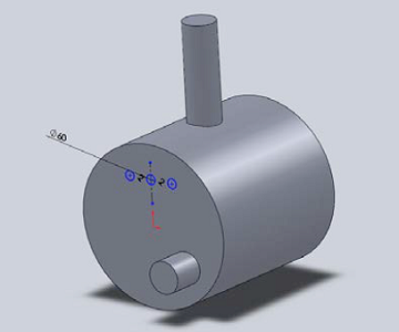
Fig.1 Geometry Design
216
ICERI 2015
2.2 Imported Geometry
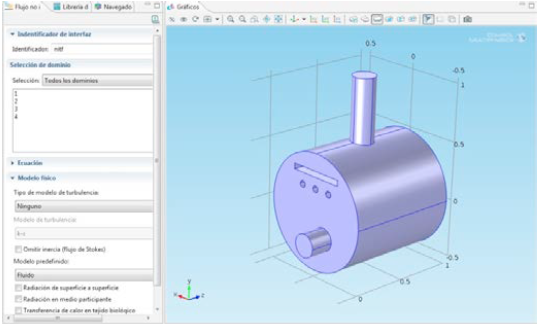
Fig.2 Geometry Recognition in COMSOL
The CAD Import Module contains a package to import geometry in the COMSOL Multiphysics
software from SolidWorks interfaces.
Once the design phase in CAD geometry submitted to multiphysics analysis, it imports to COMSOL
(Fig. 2) by applying the "geometry" command. In addition, multiphysics platform modules have the
advantage of using an option to correct any
217
ICERI 2015
issues in the contours of the imported geometry.
2.3 Use of CFD Technology
The simulation tools through the application of CFD technology provide detailed and accurate
information on velocity distributions, concentration profiles of phases, areas of high turbulence,
regions of stagnation and maps of cutting pressures of a physical system-chemical.
Using CFD it is possible to build a computational model that represents a system to study by
specifying the physical-chemical conditions of the fluid to the virtual prototype and the software
delivers a prediction of the fluid dynamics, therefore is a design technique and analysis implemented
in a computer. [2]
The main benefits of using this technology are:
− Predicting fluid properties in great detail in the domain studied.
− Design and prototyping, avoid expensive experiments.
− Process visualization and animation is possible in terms of the fluid variables.
218
ICERI 2015
2.4 Equations for flow non-isothermal
The specification of a physical or well the coupling of several physical, turns out to be an important
advantage afforded by the technology that applies. Each of the physical which includes the program,
are bounded by a system of equations that allow you to perform the analysis in the model. You can
also modify the equations which are defined in the program, either manually or with the help of a
specific module.
The analysis of the relationship of the mechanisms of transport is achieved from a system of
equations formed by the Navier-Stokes equations and the continuity equation for isothermal flow not
steady-state.
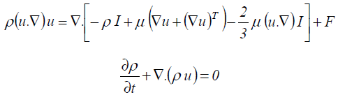
Where:  : Density,
  : Velocity flow.
  : Dynamic viscosity.
  : Identity matrix.
  : Temperature.
  : Constant.
219
ICERI 2015
In addition, the Navier Stokes equation takes into account the density constant in the term convective and discarded the effects of the turmoil, but in the study of flows should consider the assumptions about the behavior of the density versus changes in pressure and / or temperature. In the application module of the software the continuity equation is performed, in its more general version for compressible fluids, because it is the incompressible fluid as although it is permitted small changes in the density due to temperature variations. [2], [3]
2.5 Prototypes Design
It is designed two prototypes that consist of three tubes of condensation with the aim of finding the optimal conditions for operability of the computer. To do this, will be discussed in first term a condenser (prototype 1) with the tubes without any protection, and then the analysis is performed with another prototype (prototype 2) to which he incorporates a plate of shock on the tubes. Using the tool "geometry" recognizes each prototype of the condenser is performed and the proposed design: Prototype 1: The fluid enters the upper duct and passes
220
ICERI 2015
through the tubes directly with the velocity of
the same income (Fig. 3).
Prototype 2: In this case the fluid enters the condenser first hits the plate and then passes through the
tubes. Thus avoiding the direct impact of the drops on the tubes (Fig. 4).
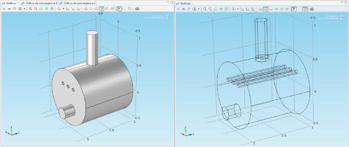
Fig.3. Prototype design 1. No strike plate.
221
ICERI 2015
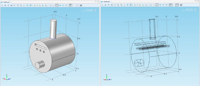
Fig.4. Prototype design 2. With strike plate.
2.6 Income 3D model parameters
After designing the prototypes shown in figs. 3 and 4, are applicable to enter the parameters of
velocity, temperatures and output pressure.
The velocity of entry of the fluid to the condenser is parameterized, ranging from 0.5 m/s to 1 m/s at a
pressure of 1 Pa relative pressure, and is caused by the download of a turbine for power generation.
The analysis is carried out in steady-state,
222
ICERI 2015
considering the incompressible flow, and moreover ignoring
the load losses. The tube temperature is 285 K (12 C) and the inlet temperature of the steam is 373 K
(100 C). The mixture of moist air pipeline emerges from the bottom, at a pressure of 0 Pa (relative
pressure) and the water is discharged in a tank of a reservoir at atmospheric pressure.
The impingement plate design is proposed to prevent the mechanical erosion of the tubes, analyzes
the pressure on them and the outlet temperatures in both prototypes.
The walls and the intermediate plate of the equipment are considered adiabatic as and is not the
subject of this analysis the condensation of the fluid, therefore, is taken at the fluid without latent heat
and not be regarded as the percentage of moisture in the fluid and these parameters objects in a later
study, and more deeper.
2.7 Meshing
Meshing Fig. 5 it is achieved with the "mesh" function of CFD simulation software. This part of the process is performed after setting the multiphysics working conditions with the need
223
ICERI 2015
to solve partial differential equations that match the presented model. To establish a meshing of geometry, first is defined the partition type (mesh) needed to perform the analysis by the finite element method. [2], [4]
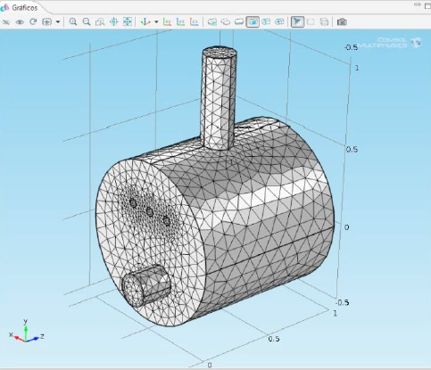
Fig.5 Meshing Geometry.
224
ICERI 2015
3 RESULTS
3.1 Prototype 1
The results obtained in the analysis of the prototype 1 are below:
In the graph in Fig. 6 are seen cutting patterns that realize the magnitude of the velocity of fluid within
the unit.
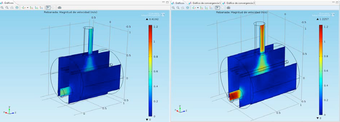
Fig.6 Plans fluid velocity. (a) To 0.5 m / s. (b) To 1 m / s.
In the 3D graphics in Fig. 7 below shows how the particles of humid air that enter the condenser
through the tubes hitting against them.
225
ICERI 2015
The mechanical erosion phenomenon shown in 3D graphics of Fig. 8 is caused by the pressure of airwater mixture fluid particles collide against the tubes. The pressure of the fluid on the condenser tubes increases four times when the velocity of the mixture is doubled. In the cases analyzed the affected area is the same.
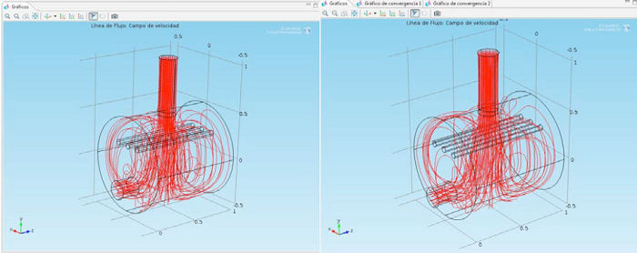
Fig.7 Lines 3D fluid flow. (a) To 0.5 m / s. (b) To 1 m / s.
226
ICERI 2015
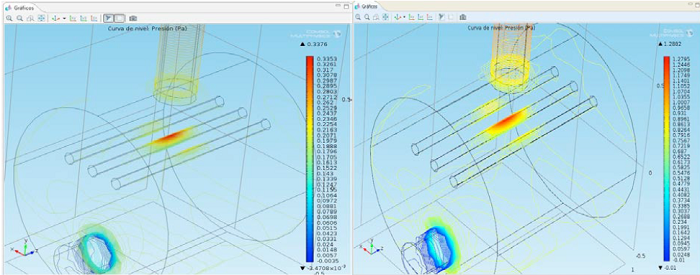
Fig.8 Contours of pressure. (a) To 0.5 m / s. (b) To 1 m / s.
In the 3D graphics in Fig. shows the temperatures inside the condenser. It can be seen that are no significant changes in the temperature gradient before a considerable variation in the velocity.
227
ICERI 2015
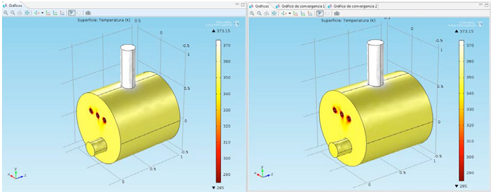
Fig. 9. 3D temperature. (a) To 0.5 m / s. (b) To 1 m / s.
3.2 Prototype 2
The results obtained in the analysis of the prototype 2 (plate with shock) are expressed below: In the graph in Fig. 10 is seen cutting patterns of behavior of the velocity of the fluid inside the computer. It is noted as the fluid hits first against the plate, going through the tubes and moves to the bottom of the condenser.
228
ICERI 2015
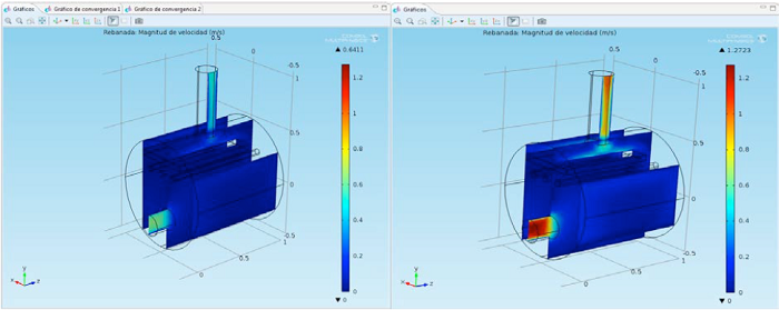
Fig.10 Plans fluid velocity. (a) To 0.5 m / s. (b) To 1 m / s.
In the 3D graphics in Fig. 11 shows the path that the particles of moist air within the condenser and the sector where the tubes are affected by the clash of the particles. In this case first the fluid collides with the plate and then passes through the tubes.
229
ICERI 2015
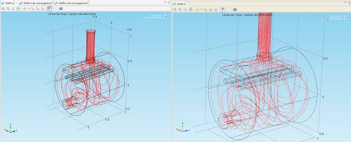
Fig.11 Lines 3D fluid flow. (a) To 0.5 m / s. (b) To 1 m / s.
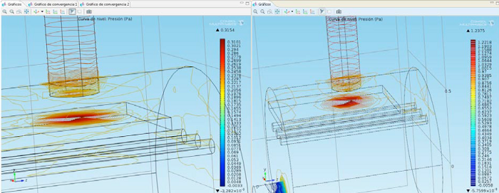
Fig.12 Contours of pressure. (a) To 0.5 m / s. (b) To 1 m / s..
230
ICERI 2015
In the 3D graphics in Fig. 12 shows the range of variation of the pressure exerted by the air-water mixture on the plate, mix colliding particles of water is observed. It is clearly seen as the fluid first hits the board and then against the tubes in the back, causing future sources of mechanical erosion that produced the consistent corrosion. The affected area is the same for both velocities of the fluid. In the 3D plot of Fig. 13 fluid temperatures are displayed within the condenser with the striking plate.
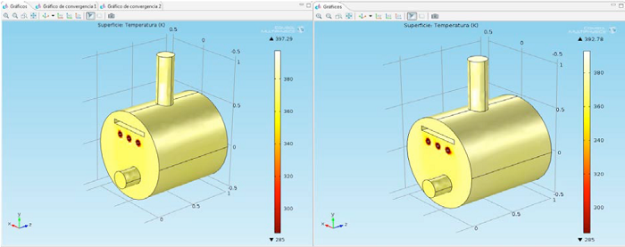
Fig.13 3D Temperature. (a) To 0.5 m / s. (b) To 1 m / s.
231
ICERI 2015
It stresses the importance of using a plate of clash of sacrifice, to prevent the flow of the fluid pressure
click directly on the tubes and consequently this will happen with the mechanical erosion of the same,
which will cause the replacement or cleaning of the tubes requiring work and cost.
Analyzes the result obtained in the graph of pressure in 3D, and it is noted that the level curves that
are generated by the pressure in the prototype 1 is on the tubes and the prototype 2 pressure should
be checked on the plate in the first instance and then dims on the back of the tubes. [5]
3.3 Comparison of the prototypes
Tables I and II shows the results obtained by comparing both prototypes and considering different physical conditions, it is noted that the temperature decreases (20 k) on the prototype 1, where the fluid travels through the tubes directly (without shock plate), as a result of this decrease in temperature, velocity of the fluid is less in this case, but the density is higher because it is located at a lower temperature. It is found that the mass flow does not vary. That is to say, the placement of the shock plate
232
ICERI 2015
generates lower temperature exchange, a higher velocity and lower density to the output.
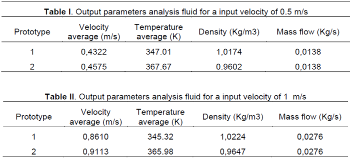
4 CONCLUSIONS
From the results obtained is observed as influences the direct impact of the fluid flow and the velocity
of the same on the tubes of the heat exchanger, to simulate the equipment by placing an intermediate
plate shock wasting the mechanical erosion flow directly from the tubes by direct contact of the
particles of water-air.
233
ICERI 2015
But a loss of efficiency in the capacitor is evident since the fluid outlet temperature does not decrease
as the prototype 1, where the flow through the tubes is directly.
We consider the limitations of the thermodynamic study for practical reasons; condensation occurs
and considers the walls and coke plate adiabatic walls. For future research these parameters can be
analyzed being an important study subject.
The integration of the design and simulation tools allow analyze various real problems that arise in
engineering, some of them with complex geometry and dynamics may not be addressed analytically.
REFERENCES
1. Tinnirello, A., Gago, E. (2013). Interdisciplinary activities to improve the learning methodology
performed in mechanical engineering degree studies. 5th International Conference on
Education and New Learning Technologies, EDULEARN 2013, pp. 5407-5416.
2. Torres, R., Grau, J. (2007). Introducción a la mecánica de fluidos y transferencia del calor con
Comsol Multiphysics. Addlink Media, pp. 87-115.
234
ICERI 2015
3. Cengel, J., Cimbala, J. (2006). Mecánica de Fluidos: Fundamentos y aplicaciones. Edit.
McGraw- Hill, 2ª Ed, pp. 471-502.
4. Comsol. Introduction to CFD (2011). Módulo, versión 4.2a.
5. Raviculé, M., Mocciaro, C., Ramajo, D., Nigro, N. (2012). Aplicaciones de fluido dinámica
computacional en la industria del petróleo desarrolladas en la dirección de tecnología de YPF.
Mecánica Computacional Vol. XXXI, pp. 3715-3739.
6. Panton, R. (2013). Incompressible flow. Edit. Wiley. 4th edition, pp. 220-257.
7. Frank, W. (2008). Mecánica de Fluídos. Edit. Mc Graw Hill 6ª edic, pp.601-646.
8. Patil, S., Kostic, M., Majumdar, P (2009). Computational fluid dynamics simulation of openchannel
flows over bridge-decks under various flooding conditions. Proceedings of the 6th
WSEAS International Conference on fluid mechanics (FLUIDS'09), pp 114-120.
235
AMATH 2015
SYSTEMS ANALYSIS AND MODELLING TECHNIQUES IN PHYSICAL DOMAINS Descargar pdf
Mónica Dádamo, Lucas D’Alessandro, Alicia Tinnirello, Eduardo Gago
Computer Basic Sciences Laboratory
Universidad Tecnológica Nacional – Facultad Regional Rosario
Zeballos 1341, Rosario, Santa Fe
ARGENTINA
atinnirello@frro.utn.edu.ar, egago@frro.utn.edu.ar
Abstract. The purpose of this work is to present the analysis of different tools for modelling physical dynamic systems, considering the complexity of the systems, pointing out the importance of their causation analysis, using different technics to model physical dynamic systems, displaying the compatibility between the traditional processing – with differential equations -, they are obtained by computer programs focus on complex and control systems -which use algebra blocks and retroaction arrows– and a new approach proposed as an alternative. It will be shown, in the development, the advantages using the Bond
237
AMATH 2015
Graph method (BG). The BG
uses physical concepts and advantage the fact that energy provides a system the dynamic of its performance,
and this is a direct consequence of the energy exchange between system components. This analysis is focused
on trying separately the resolution technic; as the case may be mathematical, numerical or computational; so
that the knowledge acquired does not depend on outdated methods or technologies.
Keywords: Modeling, simulation, multidisciplinary, computational mathematics.
1 INTRODUCTION
In engineering, we associate the analytical vision, found in classical physics, with the systemic approach, an essential component of professional modelling and simulation software together with other computer tools integrating basic sciences with the engineering activity.
238
AMATH 2015
This new approach includes the concepts of
causation, retroaction and ports, as well as the
emergent vision of programming paradigm focused
on objects in order to create bases that allow us
choosing between different resolution techniques,
also adding those concepts that enable the resolution
of systems with more than one degree of freedom,
non-linear, with multiple inputs and outputs.
Linear time invariant dynamical systems are
gradually developed to study the model that
represents the early feedback stage in simple
description of physical phenomena. This approach
facilitates software engineering professionals when
designing systems with controllers, where the
feedback is considered a main feature [1].
The advantages of the Bond Graph method
application will be demonstrated; it uses physical
concepts and takes advantage of the fact that energy
provides a system the dynamic of its performance,
and this is a direct consequence of the energy exchange between the components of a system. BG
only uses two types of variables, named conjugated
variables of power: effort (e) and flow (f), both
defining the interaction of power, remaining that the
result of them is power.
239
AMATH 2015
2 MOTIVATION AND OBJETIVE
These days, characterized by scale, uncertainty and new degrees of complexity, a lot of challenges need solutions which are out of reach of an only disciplinary thought [2]. The purpose of this work is to present the analysis of different tools for modeling physical dynamic systems, showing the compatibility between the traditional processing -with differential equations-, the obtained by computer programs focus on complex and control systems -which use algebra blocks and retroaction arrows- and a new approach proposed as an alternative. This analysis is focused on trying separately the resolution technic; as the case may be: mathematical, numerical or computational; so that the knowledge acquired does not depend on outdated methods or technologies. We want to highlight the portability of the model; trying the same pattern of analysis be applicate regardless of the character of the system (mechanical, electrical, hydraulic, etc.)
3 METHODOLOGICAL BASES
In the review of systems and simple phenomena we could
240
AMATH 2015
consider one effective way of dealing with subject of study. It is connected directly with the comprehension of the topic. In complex systems, the relation between the operational knowledge and the justification and explanatory areas is potentially more diffuse. We can notice one example in the analysis of the simple dynamic systems such us a mass-spring system (M_S) either an electrical system R-L-C: In these cases, it is easy to get the model through an Ordinary Differential Equation (EDO) raising its constitutive and structural relations Fig.1.
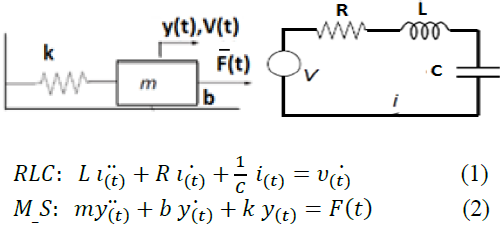
Fig.1 Dynamic systems and EDOs
An order n EDO can be rewritten as n EDOs order 1 system,
241
AMATH 2015
named States Equations. On this
way, It is defined 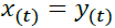 ,
, 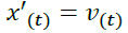 for the
equation (1) the system is:
for the
equation (1) the system is:
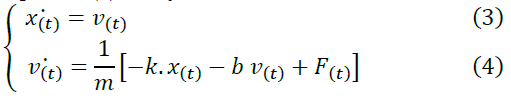
Where x(t), y(t), are called state variables.
In circuit RCL, defining 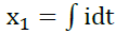 ,
, 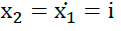 we get the system:
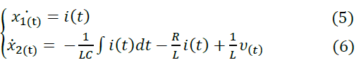
Where ,  are the state variables.
Even though the Continuous Systems are
represented through differential equations models, it
is very difficult to obtain the right equations directly
when the model grows up in complexity for the
following reasons:
- The equations systems cannot be coupled to
get complex models from simple models.
242
AMATH 2015
- To get the EDO, from the consecutive and
structural relations, it is necessary algebraic
effort.
- The obtained models have not got visual
similarities with the originals schedules.
That is why to obtain continuous systems models
it is advisable using graphical languages with
Diagram Blocks (DBs). The DBs simplify the
algebraic manipulation of constitutive and structural
relations.
Then, we consider two systems separately, a CC
engine (Fig.2a) and a pulley (Fig.2b), and their
respective models are made with DBs (Fig.3d). In
the event of couple mechanically the systems
(Fig.2c): Is it possible to obtain DB of the new
system coupling the partial DBs of the engine and
pulley?
243
AMATH 2015
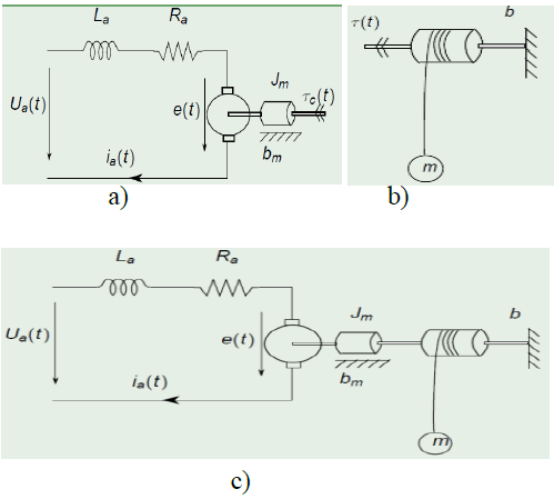
244
AMATH 2015
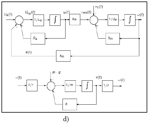
Fig.2 Dynamic systems, a) cc engine, b) pulley, c) engine + pulley, d) modelling with DBs
In Fig.2d is shown it is not possible, since the
variable (t), which links the systems, appears as
input in both DBs.
In addition to establishing mathematic relations,
the DBs establish causal relations between the
variables. For this reason, each sub-system sees the
interaction variables as ‘input –
245
AMATH 2015
output variables’. If
two sub-systems see their interaction variables with
the same causality, there will be a causal conflict
and the DBs cannot be coupled [3]
A formalism to couple sub-systems must be noncasual
and here is where the concept of bond graph
comes up. It constitutes an important tool to obtain
mathematical models from physical concepts such
as the exchange of energy in the sub-systems.
This method was developed by Henry M.
Paynter. In contrast to modelling with other
methods, BG uses physical concepts and it makes
use of the fact that energy provides a system the
dynamic of its performance, and this is a direct
consequence of the exchange of energy between the
system components. In this way the BG graphical
language is a tool to get mathematical models from
that exchange, representing instantaneous power
flow, transformation, storage and dispersion energy
phenomena’s and the structural relations, in
a unified manner. BG uses only two principal
variables, named power conjugated variables: effort
(e) and flow (f), both defined the interaction of
power, taking into account that the result of them is
the power.
246
AMATH 2015
4 DEVELOPMENTS
In engineering, the modelling of systems energetic
performance involve the breakdown of a system in
elementary conceptual sub-systems, which represent
basic physical processes and determinate the system
performance from the energetic point of view. This
basic physical process can be classified as: storage
processes, transporting and distributing, dissipation,
and exchange of energy.
The final product of the breakdown could be
represented with a connecting graphs diagram. On
this way, a priori the system for modelling is
intended as a net which interconnects basic
elements. These elements, storage, dissipate or
transform the energy. When these interact with each
other, the product is a bidirectional and non – causal
flow. The components of the system interact with
each other determining the dynamic of the system.
In the same line of though, it is considered one
fundamental fact when two systems (S1,S2) or
elements interact, none of them can impose both
variables. If one of them sends an effort signal (power, voltage) the other one answers with a flow
signal (speed, current); in inverse, if one of them
247
AMATH 2015
impose flow, the other one determinate the effort (Fig. 3).
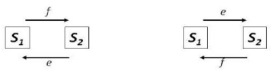
Fig.3 Signal flow in a simple Bond Graph
In the BG notation is used an arrow named Bond to represent the power flow between two subsystems. Each arrow has two associated variables (“e” and “f”), the product of these variables is the power and the arrow`s way just indicate where is going the positive flow of energy, it does not indicate the flow way and the effort way. (Fig.4)
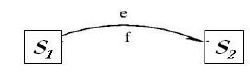
Fig.4 Energetic relation between two elements by using BG.
248
AMATH 2015
Table 1: Variables of effort, flow, moment and displacement in different physical domain
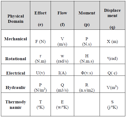
The physical meaning of the effort and flow variables will depend on the physical domain where the system of study be established. Apart from the mentioned variables, the method
249
AMATH 2015
uses two more variables, named energetic or dynamic. These variables are: the integral flow in time called displacement q(t> and the integral effort in time P(t) called moment:
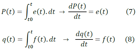
In Table 1 we can see the meaning of these variables in different physical domains.
4.1 Basic elements of Bond Graph
Then, there is a group of basic elements used to
model each system. These elements appear as
elementary components of system, representing
their mathematical idealization.
The BG technique makes possible, as a result of
the defined variables classification, the
representation of models belonging to any physical
domain only by using a small amount of elements.
Resistive elements R: they have a static relation
250
AMATH 2015
between the effort and flow in which there is energy
loss. These elements can represent electric
resistances, shock absorbers, friction efforts, head
loss in pipes, etc.
Capacitive elements K: They can be modelled as
flow stored elements. These elements are capable of
storing energy and return it to the system without
losses. A capacitor can represent springs, torsion
bar, electric capacitors, hydro pneumatic
accumulators, etc. Contrary to resistive elements,
the capacitive ones relate the effort associated to the
graph with the displacement produced. Whereas the
displacement is defined as the flow integral in the
time, in the capacitive elements:
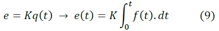
Inertial or inductive elements L: They can be modeled as effort stored elements. These elements are capable of storing energy and return it to the system without losses and they relate the flow with the P variable defined as the effort integral in the time. The condition is met:
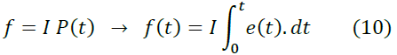
251
AMATH 2015
An inertial element can represent electrical inductors, masses in mechanical systems, etc. Fig.5 shows the representation with BG method of different elements in an electrical system.
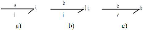
Fig.5 Representation with BG method of the different elements for an electrical system: a) Resistive b) Inductive c) Capacitive.
Union nodes: In those points of the systems, where there are one or some energy inputs and one or some outputs, it is produced a node which complied with the principle of energy conservation. It met:
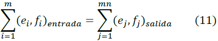
There are two types of unions named ‘type 0’ or
‘type 1’.
Union 0: It is also called parallel connection. All
graphs connected to this union, have the same effort,
and the product of the sum of flows is zero. These
connections represent
252
AMATH 2015
mechanical systems that share the same effort, electrical systems that share the same tension, etc. Union 1: It is also called serial connection. All graphs connected have the same flow and the product of the sum of the efforts is zero. These connections represent mechanical systems that share the same speed, electrical systems that share the current, etc.
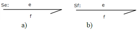
Fig.6 Representation in BG method of flow elements: a) of effort b) of flow.
Source elements: They provide power to the
system. This power can be provided through a flow
or an effort, in such a way there will be two kinds of
sources: known effort (excitation force in
mechanical systems, voltage generators in electrical
systems, etc.) and known flow sources (electrical
current sources, hydraulic pump as flow rate source,
etc.). Fig.6 shows the flow representation in BG.
Transforming elements: They transmit power
variables with a
253
AMATH 2015
scaling defined by its module, and they preserve the power. This element represents electrical transformers, levers in mechanical systems. In BG notation, its representation is shown in Fig.7.
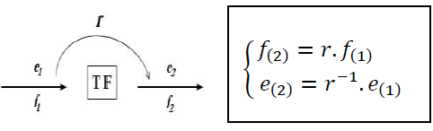
Fig.7 Transforming elements, BG representation and Variables relation.
The symbol r indicates the scaling module and the arrow shows the transforming direction. Fig.8 shows the implementation of these concepts in the modeling of different systems:
254
AMATH 2015
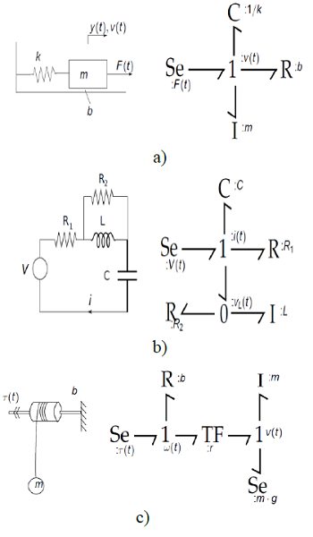
Fig.8 Modeling of systems with BG notation. a) M_S b) RCL combined c) pulley
255
AMATH 2015
Taking up the example of the pulley system
coupled to the CC engine, which results in the
causality conflict as it attempts its coupling through
the modeling technic with diagram block, we will
try to attach both sub-systems coupling directly their
respective BG models in the same way we attempt
with the DBs models.
Whereas the pulley model obtained of picture 8c,
the BG model of CC engine is carried out (Fig.9).
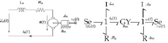
Fig.9 BG modeling of CC engine.
Coupling both systems (Fig.10)
256
AMATH 2015
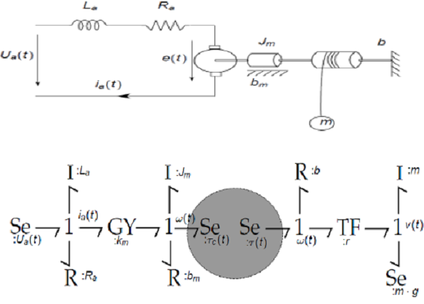
Fig.10 BG modelling of CC engine + pulley.
Looking at the shaded area in the BG of Fig.10 and assuming the non-casual nature of BG, it is possible to couple directly both systems joining the two links which have 𝜏(𝑡) as a variable, in this way to get the complete model of the system. It is shown in Fig.11.
257
AMATH 2015
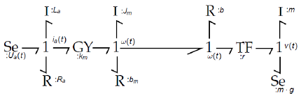
Fig.11 CC modelling of CC engine + pulley coupled.
The previous BG has all the system equations in a non-casual way and this absence of causality allows to couple subsystems in a trivial manner.
4.2 Obtaining state equations from BG –
Causality assignation.
One of the main objectives from doing an analysis of a Bond Graph model is the causality assignation. This involves the determination of which systems provide the flow or the effort. In BG notation it is done with a vertical bar, named causal trace. It is collocated in the end where the flow inputs to the graph, or in other words, in the end where there is the output effort. Fig.12_a shows the causality between two elements A and B. Effort flows from A element to B. It is indicated by the causality bar in the right end of the link. Fig.12 shows the opposite case.
258
AMATH 2015
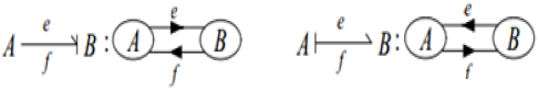
Fig.12 Causality between two elements.
One advantage of BG is there are a lot of
procedures to get the causality assignation, for this
reason this task is reduced to a sequential and
simple action, as long as the ‘causal dependence’ of
each one of the basic elements below be respected.
These elements are classified by the causal
assignation point of view, as follow:
Fixed Causality: They are the flow source ones
(causality flow) and effort source (causality effort).
By definition, they provide information of one kind
or another.
Indistinct causality: Resistive elements.
Preferred causality: They are energy stored
elements (capacitive or inductive) which can have
integral or differential causality in order to the
relation between the flow and the effort. Integral
causality is more preferred than differential
causality because of the integration is a more
efficient computational procedure.
Multi ports with restricted causality:
Transformers and unions. It
259
AMATH 2015
is denominated in that
way because imposing the causality of one of its
bonds, the causality of the rest is obtained. Once
the BG causality is determinate, we have to identify
the state variables. They are the stored variables
with integral causality. Once the state variables are
obtained, it is possible to get from BG the system
equations directly, following its causality and using
the laws of the components [4-5].
The importance of this modeling tool is that once
the Bond Graph of the system has been obtained, all
the following steps until obtaining the equations, are
fully algorithmic. It is possible, in this algorithmic
way, to get a diagram block and/or the related state
equations from the BG. The causal assignment
procedure (SCAP), its variations MSCAP and
RCAP (Relaxed causality Assignment Procedure),
are a few of the many algorithmic procedures
developing to assign causality and to get the
equations of systems modeled by Bond Graph.
There are software capable of manipulate and
simulate BG: 20Sim, Dymola, PowerDynaMo and
more.
260
AMATH 2015
5 CONCLUSIONES
This analysis focus on trying separately the resolution technique, as the case may be: mathematical, numerical or computational, so that the knowledge acquired does not depend on outdated methods or technologies. We want to highlight the portability of the model; that the same pattern of analysis may be applicate regardless of the character of the system (mechanical, electrical, hydraulic, etc.). This new approach about system analysis makes it possible to simplify the variables in complex systems with different components. It breaks with the ‘unique model of thought’ and prepares the future engineers in the management of an actual complexity, this day, unavoidable.
REFERENCES
1. A. Tinnirello, M. Dádamo, E. Gago, Integration
techniques in mathematical application projects
for mechanical engineering, 6th International
Technology, Education and Development
Conference, 2012, pp. 1844-1850.
261
AMATH 2015
2. G. Van Del Linde, ¿Why is it important
interdisciplinary higher education? Journal of
University Teaching, Vol.IV. No. 8, 2007.
3. E. Kofman, S. Junco, Quantized Bond Graphs:
An Approach for Discrete Event Simulation of
Physical Systems, Proceedings of International
Conference on Bond Graph Modeling and
Simulation ICBGM’01, 2001, pp. 369–374.
4. G. Romero, J. Félez, J. Maroto, J. Cabanellas,
A minimal set of dynamic equations in systems
modelled with Bond Graphs. Proceedings of
the Institution of Mechanical Engineers, Part I,
Journal of Systems and Control Engineering,
Vol.CCXXI, No.1, 2007, pp.15-26.
5. G. Esperilla, J. Félez, G. Romero, A. Carretero,
A model for simulating a lead acid battery
using Bond Graphs. Journal of Simulation
Modelling Practice and Theory, Vol.XV, No.1,
2007, pp. 82-97.
6. G. Romero, Procedimientos optimizados
utilizando métodos simbólicos para la
simulación de sistemas dinámicos mediante
Bond-Graph, Tesis Doctoral, 2005.
7. I. Roychoudhury , M. Daigle, G. Biswas, X.
Koutsoukos, Efficient
262
AMATH 2015
Simulation of Hybrid
Systems: A Hybrid Bond Graph Approach,
Simulation: Transactions of the Society for
Modeling and Simulation International, Vol.
LXXXVII, No.6, pp. 467-498, 2010.
8. V. Damic, J. Montgomery, Mechatronics by
Proceedings of the European Computing
Conference Bond Graphs, Springer, 2003.
9. I. Roychoudhury, G. Biswas, X. Koutsoukos,
Using Factored Bond Graphs for Distributed
Diagnosis of Complex Systems, Proceedings of
the 9th International Conference on Bond
Graph Modeling and Simulation, 2010, pp. 11-
18.
10. W. Borutzky, Bond Graph Modelling of
Engineering Systems. Theory, Applications and
Software Support, Springer, 2010.
263
Ingeniería Matemática: Modelado y Simulación de Sistemas Complejos en
el contexto de las Tecnologías Básicas y Aplicadas
Homologado por la Secretaría de Ciencia y Tecnología bajo la identificación Nº UTI3793TC
Fecha de inicio: 01/05/2016
Fecha de finalización: 30/04/2019
IJPS 2016
ANALYSIS AND PREDICTION OF ELECTRIC FIELD INTENSITY AND POTENTIAL DISTRIBUTION ALONG INSULTOR STRINGS BY USING 3D MODELS Descargar pdf
Alicia Tinnirello, Eduardo Gago, Lucas D’Alessandro, Mariano Valentini,
Computer Basic Sciences Laboratory
Universidad Tecnológica Nacional – Facultad Regional Rosario
Zeballos 1341, Rosario, Santa Fe
ARGENTINA
atinnirello@frro.utn.edu.ar, eagago@gmail.com
Abstract. This The paper presents the development of three-dimensional models for the study of the electric field intensity and the potential distribution in insulators strings of an electrical system using the finite element method, and through a multiphysics platform is performed the resolution of physical systems, modelling and simulations. The design of models allows the calculation and simulation of the potential distribution and electric field intensity on insulators under different conditions of
267
IJPS 2016
operation by enabling the analysis of the behavior against variations in conditions and factors involved in its functioning, as well as the evaluation of strategies for the mitigation of its consequences. In many high voltage applications corona discharge is seen as an unwanted side effect. Corona discharge from high voltage electric power transmission lines constitutes an economically significant waste of power for utilities. This analysis allows predicting possible future outputs of service of power lines due to failures of isolation and thus anticipating and scheduling preventive solutions.
Keywords: design, insulators, corona discharge, electric field, prediction.
1 INTRODUCTION
In transmission and electricity distribution systems insulators strings operate under mechanical, electrical efforts and environmental constants such as own ongoing efforts caused by voltage operation and weight of the elements associated
268
IJPS 2016
with the chains (cables, brackets, accessories), transient efforts as lightning, operation switches, contamination in the chains, wind temperature changes, additional charge by presence of ice, rain, etc.
All of these factors affect the normal performance of the lines leading to the emergence of phenomena such as corona discharge and partial discharge. These phenomena produce consequences such as loss of power, generation of light, audible noise and interference, vibration, deterioration of materials, generation of ozone, nitrogen oxides and moisture between others and, if reaches certain importance, produces corrosion in drivers because of the formed acid [1].
Currently both the University and the professional scope of electrical engineering the study of these phenomena is carried out by analytical calculations based on empirical methods. These calculations allow us to determine the potential gradient for which appears ionization on the conductor surface called surface critical gradient under certain operating conditions from which it is possible to calculate the losses and other consequences due to corona discharge or verify the levels of tension and line conditions, but is not analyzed the behavior
269
IJPS 2016
and distribution of the field and electric potential.
The electric field behavior and potential distribution has various options for its analysis which are: analytical methods through a simplified equivalent circuit, the pilot based on the measurement of fields and the numeric which approximate the solution of the problem through the implementation of numerical methods that solve the equations that define the behavior of the electric field. The first option does not allow an effective evaluation of the field and the distribution of the electrical potential, and the complexity of the model makes it difficult to obtain a solution. Experimental though effective involve high costs and sometimes the measurement methods can affect the natural behavior of the phenomenon. On the other hand, the application of numerical methods accompanied by progress in computational systems that use these techniques for solving allows complex studies of electromagnetic phenomena becoming a useful tool, flexible and less costly with respect to experimental methods.
One of the first researchers of the study of the discharge corona was F. W. Peek, who carried out his first experiments with a line of 275 m in length, powered by a 200 kV single-phase
270
IJPS 2016
transformer since 1912. Diameters of wires analyzed by Peek experimentally were from several millimeters to an inch [2]. Subsequently, a large number of researchers is interested by this phenomenon, among them L. B. Loeb who headed one of them groups of research that more have contributed to the knowledge of the corona discharge. Loeb published in 1965 the book entitled "Electrical coronas" which is still considered a very important reference work [1]. The works and research oriented the analysis of the field electric in insulators of lines electric, are these of glass tempered, porcelain or synthetic through numerical methods due to [3], who define a method to determine an electrical field of low frequency in standard contaminated insulators, whereas models axisymmetric are considered and applying finite element method.
Rasolonjanahary analyzes the three-dimensional behavior of insulators contaminated using the numeric method of border elements establishing a theoretical formulation and comparing the results with obtained in analytical and experimental way [4].
Due to the continuous advancement in computer systems, can be currently studies extremely complex for electromagnetic phenomena using experimental and numerical techniques. The
271
IJPS 2016
study and analysis of the electric behavior in insulators chains of glass tempered, porcelain and of others types as synthetic through the application of numerical methods allow the insulating design, as well as study the dimensioning of transmission structures (towers and posts) and the configuration of lines of transmission, influencing directly in the optimization of costs and improvements in the performance of transmission systems [5].
2 APPLIED METHODOLOGY
Through three-dimensional models is evaluate and computationally analyzed different operation conditions of insulators strings that constitute lines of transmission and distribution of electric energy. Insulators are used as support and drivers, at the same time holding them isolated from earth [6]. The most common material used for insulators is the porcelain shown in Fig. 1, and glass and synthetic materials such as epoxy resins.
272
IJPS 2016
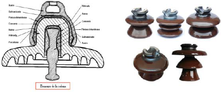
Fig.1 Porcelain electric insulator
Strings made of insulators are used in high and medium voltage by a variables number of them dependent from voltage operating (Fig.2).
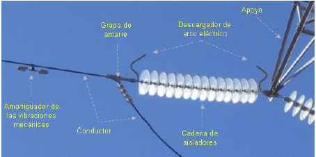
Fig.2 Insulator stringsr
273
IJPS 2016
When the electric field or potential gradient reaches the "dielectric strength of air" (approximately 30 kV/cm at normal atmospheric pressure), the air is ionized, becomes conductive and produced a local discharge. This phenomenon is accompanied by a luminous glow which comes from the name of corona discharge. In addition, produced losses of energy, an easily perceptible hum and noise on radio and television in the vicinity of the area where the phenomenon is located. Ozone is also produced in the presence of moisture, nitrous acid, which brings as a consequence the corrosion of conductors if the phenomenon is intense. The surface gradient necessary to achieve the threshold corona in the gas surrounding a smooth cylindrical conductor, is called visual critical gradient or gradient of initiation, Ev. The level Ev on the surface of the conductor means that at a certain distance from that surface breakdown level required activate the download process and the beginning of the luminous manifestations has been reached [7].
The calculation of the critical or initiation gradient, from which there are downloads of the type corona is of great importance to evaluate the consequences of this phenomenon. The critical
274
IJPS 2016
gradient is a function of the conductor diameter , the condition of its surface and the relative density of the air which in turn depends on the pressure and temperature . Peek, obtained empirically formula that is the most used for the calculation of the critical gradient in cylindrical conductors. The critical gradient "Ec", kV tip/cm, is expressed as:
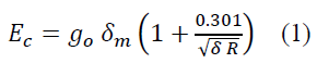
Where
 : disruptive critical gradient of air
  29.8 kVpunta / cm.
 : conductor radio, en cm.
 : relative air density
 : state superficial coefficient
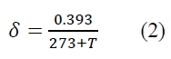
Where P air pressure, en mm Hg, and T air temperature, in °C. The analysis and evaluation of the models was conducted using the computational tool Comsol Multiphysics. This is a package of software analysis and resolution by e.m.f for various
275
IJPS 2016
physical applications and engineering, especially coupled phenomena, or Multiphysics.
3 MODELLING A 3D INSULATOR STRING
3.1 Protothype in CAD and geometry
The equipment design is developed in CAD (Fig.3.a), this design is imported to COMSOL (Fig.3.b). Multiphysics platform modules have the option of correcting any inconvenience in the contours of the imported part.
276
IJPS 2016
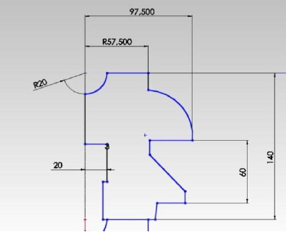
Fig.3 a) Geometric design in CAD
277
IJPS 2016
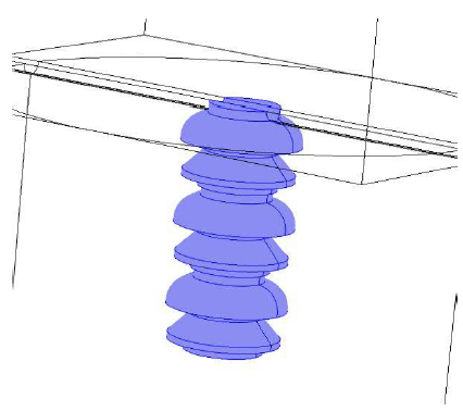
Fig.3 b) Geometry imported in COMSOL.
3.2 Using AC/DC Technology
The module AC/DC allow the possibility to built a computacional model that represent a ssytem under study by specifying the physical conditions of the virtual prototype and software delivery prediction of electric, magnetic and electromagnetic fields, so it is a design and analysis technique
278
IJPS 2016
implemented in a computer. [8]. The main advantages that brings the use of this technology are: the electric field prediction, the design and protothype system avoiding experiments of high cost, the visualization and the animated system in the variables terms modifying the components properties and the environment.
3.3 Meshing Sequences
To solve the proposed moddels we must make a mesh geometry. The meshing of Fig. 4 is achieved with the function "mesh" CFD simulation software, this part of the process is of utmost importance and it is always done after adding and defining multifisics conditions, it is here in which defines the type of mesh necessary for the analysis by finite element.
279
IJPS 2016
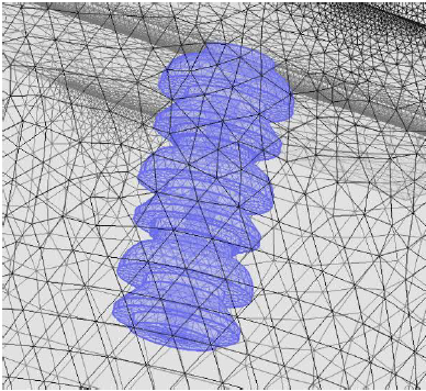
Fig.4 Model meshed
3.4 Simulations sequences
After design the chain of insulators model to study, is possible carry out a without number of simulations of the same facing under different conditions of operation, modifying parameters of interest e involved in the training of the phenomena in study. Below are some of the conditions simulated in the chain of
280
IJPS 2016
insulators on a line of 33kV corresponding to those used for the distribution of energy in medium voltage in Argentina.
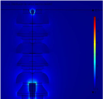
Fig.5 Electric field distribution in porcelain insulator
281
IJPS 2016
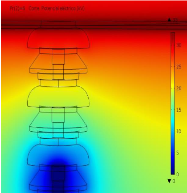
Fig.6 Potencial Electric
282
IJPS 2016
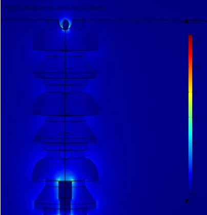
Fig.7 Distribution of electric field in insulator of ethyl propylene.
283
IJPS 2016
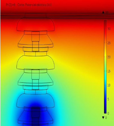
Fig.8 Potential electric.
The Fig. 5, 6, 7 and 8 show respectively the distribution of field and potential electric of the chain of insulators when this is composed of insulators of porcelain and ethyl-propylene.
284
IJPS 2016
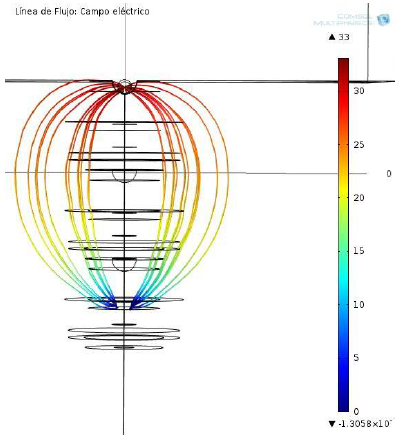
Fig.9 Flow lines of electric field in porcelain insulator.
285
IJPS 2016
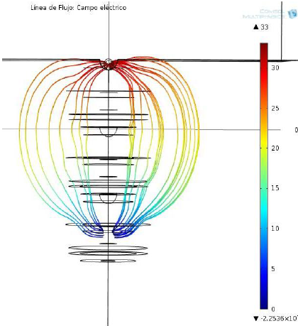
Fig.10 Lines of flux of electric field in ethyl propylene insulator
Fig. 9 and 10 shows the distribution of the flow lines of the electric field in both cases.
The electric field through the length of arc of the insulator where supports the driver for different materials, which differ in the electric permittivity: synthetic material  , ceramic
  , glass
  are
are
286
IJPS 2016
analyzed, Fig. 11 and 12. One of the alternatives to reduce the electric field in this area is to add a semi-conducting screen between conductor and insulator. The Fig. 13 and 14 shows the evaluation of such alternative.
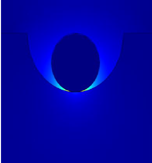
Fig.11 Level surface of Electrical field in length of arc for different materials
287
IJPS 2016
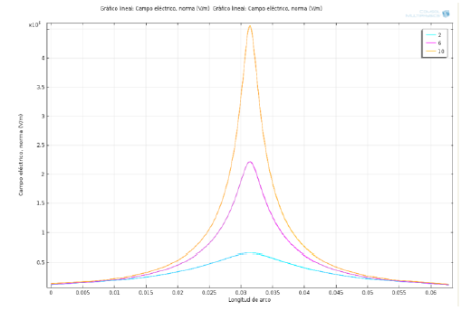
Fig.12 Electrical field in length of arc for different materials
288
IJPS 2016
Fig.13 Level surface of Electrical field in length of arc for different materials with semiconductor plate.
289
IJPS 2016
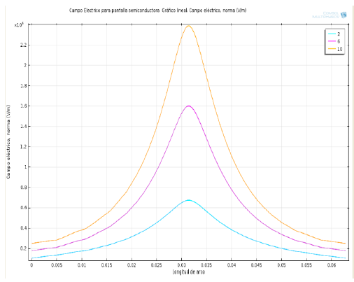
Fig.14 Electrical field in length of arc for different materials with semiconductor plate.
The distribution of electric field in the case of an insulator damaged within the chain is simulated in Fig. 15 and 16.
290
IJPS 2016
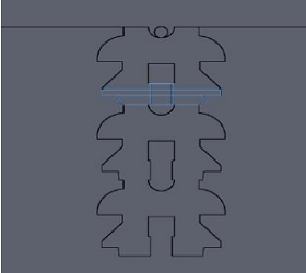
Fig.15 Level surface of Electric field distribution for damaged string insulator
p>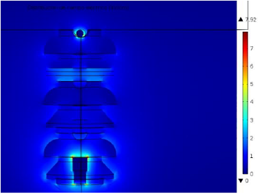
Fig.16 Electric field distribution for damaged string insulator
291
IJPS 2016
Through a contour area, whose material properties can be configured easily, in the upper part of the elements that make up chain could be analyzed the effect of them front of deposited pollution or face the effect of water product of rain. This last case is presented in Fig. 17 and 18.
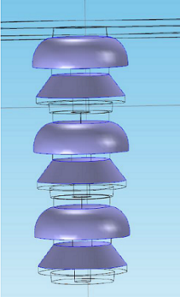
Fig.17 Distribution of Electric field for the chain of insulators with wet surface.
292
IJPS 2016
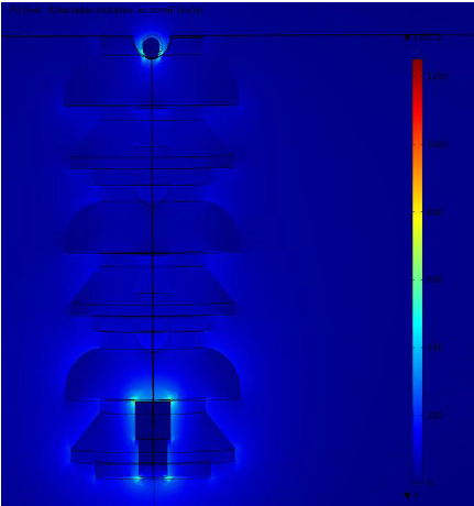
Fig.18 Distribution of electric field for the chain of insulators with wet surface.
5 MODELING RESULTS AND DISCUSSION
Use materials of low permittivity, ethyl-propylene case with
293
IJPS 2016
respect to the ceramic or glass, involves a considerable decrease in the electric field; made desirable to mitigate the consequences of the corona effect and the partial downloads , Fig. 5 and 6.
An insulator damaged in the chain involves the loss of dielectric uniformity of the same generating a sudden change in the nature of the insulation and consequently an increase in the field in a relatively small region, presenting conditions favourable for the occurrence of partial discharges, Fig. 10.
Using a semi-conducting screen between the insulator and the driver allows us not only reduce the electric field, but it becomes more uniform around the point of contact between the insulator and conductor, Fig. 9.
All cases show that insulating contact point - driver is the increased intensity of field so this area is the greater issue of corona discharge.
Edges located at the ends of the insulator have the highest values of field because they are areas where high potential gradients are generated. This fact is important to analyze now that it is a propitious area for the initiation of surface discharges that can have outcome on the dielectric breakdown of the insulator, which is known as flutter and has the consequence
294
IJPS 2016
of the outputs of services from electrical power lines.
The presence of water on the surface of the insulator generates a reduction of the dielectric strength of the same with an electric field more intense in a damp insulator that being dry as shown in Fig. 11. On the other hand, the products of rain moisture favors the appearance of disruptive discharges through the air due to the ionization of the same reason of humidity.
A layer of humidity on the insulator implies an increase in the conductivity of the same favoring the emergence of currents that outlined the outside of it.
4 CONCLUSION
The corona and partial discharges occur in non-uniform fields, in areas with large field intensities and is favored by the presence of humidity or contamination in the insulators, so these should be issues to take into account in the design of the chains according to the conditions in which it will operate the same.
These discharges in an insulating material usually begin in hollow filled with gas within the dielectric. After a partial
295
IJPS 2016
discharges occurs a progressive deterioration of insulating materials, causing the rear insulation fault and subsequent exit of the line service.
The implementation of computational tools as CDF, for the analysis and simulation allows great versatility in the study of different conditions of operation in order to predict the behavior of the system under different conditions and so to program preventive actions for avoid consequences.
REFERENCES
1. S. Hernandez Morales, Martinez Sanchez, A, Influencia de la humedad y contaminación sobre aisladores epdm-siliconados. Tesis doctoral, Escuela Superior de Ingenieria Mecanica y Electrica, México, 2009.
www.sistemamid.com/download.php?a=77341
2. S. Ilhan, A. Ozdemir, Effects of corona ring design on the electric field intensity and potential distribution along an insulator string, Proceedings of 5th International Conference on Electrical and Electronics Engineering, Vol.1, No1, 2007, pp. 12-17.
296
IJPS 2016
3. Asenjo, E., Morales, N., Valdenegro, A., Solution of low frequency complex fields in polluted insulators by means of the Finite Element Method. Journals and Magazines IEEE Transactions on Dielectrics and Electrical Insulation, Vol. 4, No. 1, 1997, pp. 10-16.
4. J. Rasolonjanahary, Computation of Electric Fields and Potential on Polluted Insulators using a Boundary Element Method. Journals and Magazines IEEE Transactions on Magnetics. Vol. 28, No. 2, 1992, pp. 1473-1476.
5. Zhao, T., Comber, G., Calculation of Electric Field and Potential Distribution along Nonceramic Insulators Considering the Effects of Conductors and Transmission Towers. Journals and Magazines IEEE Transactions on Power Delivery, Vol. 15, No. 1, 2000, pp. 313-318.
6. K Kiousis, A. Moronis, E. Fylladitakis, Finite Element Analysis Method for Detection of the Corona Discharge Inception Voltage in a Wire-Cylinder Arrangement, Recent Advances in Finite Differences and Applied & Computational Mathematics, WSEAS Press, 2013.
7. K. Kantouna G. Fotis et al., Analysis of a Cylinder-Wire-Cylinder Electrode Configuration during Corona Discharge, Latest Advances in
297
IJPS 2016
Information Science, Circuits and Systems, WSEAS Press, 2012.
8. A. El Dein, Prediction of Egyptian 500 kV Overhead Transmission lines RadioInterference by Using the Excitation Function, Proceedings of WSEAS Transactions on Power Systems, Vol.9, No.1, 2014, pp. 479-485.
298
IJCE 2016
DIAGNOSIS OF ROTOR FAILURES CURRENT POWER INDUCTION MOTORS BY SPECTRAL ANALYSIS METHODS Descargar pdf
Alicia Tinnirello, Eduardo Gago, Lucas D’Alessandro, PaolaA Szekieta
Computer Basic Sciences Laboratory
Universidad Tecnológica Nacional – Facultad Regional Rosario
Zeballos 1341, Rosario, Santa Fe
ARGENTINA
atinnirello@frro.utn.edu.ar, eagago@gmail.com
Abstract. Nowadays many tasks which a modern industry carry out, are performed by induction motors, becoming the core of most common industrial processes. The operators of induction motor drives are under continual pressure to reduce maintenance costs and present unscheduled downtimes which result in loss of production and financial income. Many operators now use online condition-based maintenance strategies in parallel with conventional planned maintenance. Motor current signature analysis (MCSA) is the online analysis of current to
299
IJCE 2016
detect faults in a three-phase induction motor drive while it is still operational and in service. In industrialized countries between 40% and 50% of all energy produced is generated for consumption of these engines. As the market of these engines has grown and continuous and efficient monitoring has become indispensable, companies have to progressively invest on methods of preventive maintenance based on prediction of failures on operation programs. This type of maintenance, also known as condition-based maintenance (CBM) is an approach which changes the functioning condition and / or team performance when making decision as repairs or replacement. The goal of CBM is to minimize the total cost of inspections and repairs to collect and interpret data related to the operating condition of critical components of a computer continuously (online) or discontinuous (over time). This paper focuses only on fault detection by broken bars in squirrel cage induction motor and more specifically in the task of signal analysis and diagnosis, using LabVIEW software platform by a method which applies the Fourier Transform for spectral analysis of the feed stream.
Since our interest is focused on signal analysis, rather than on the acquisition of technical data, the choice of LabVIEW as a
300
IJCE 2016
deployment platform which facilitates the acquisition and signal conditioning, was intentional to carry out tests with signals stored provided by Massey Technical Service Laboratory.
MCSA is presented as an excellent alternative online monitoring and non-invasive to diagnose many faults in induction motors becoming a tool to consider in predictive maintenance schemes.
LabVIEW allows a user- friendly implementation and facilitates the collection, processing, storage of data, facilitating the generation of reports and statistics.
Keywords: MCSA; Induction Motors; LabVIEW; broken bars
1 INTRODUCTION
Nowadays, as many of the tasks that a modern industry must carry out are performed by induction motors, induction motors have become the core of most common industrial processes.
In industrialized countries between 40% and 50% of all energy produced is used for these machines [1]. As the market for these engines has grown to have control and continuous and efficient
301
IJCE 2016
monitoring has become indispensable, companies have to progressively invest on methods of preventive maintenance based on prediction of failures on operation programs. This type of maintenance, also known as condition-based maintenance (CBM) is an approach which changes the functioning condition and / or team performance when making decision as repair or replacement [2]. The goal of CBM is to minimize the total cost of inspections and repairs when collecting and interpreting data related to the operating condition of critical components of a computer, continuously (online) or discontinuous (over time). Thus the CBM reduces costs of inspection and repair by allowing the identification of those faults when they are close to occur. In this case, repairs are based on the degradation of equipment preventing costly repairs when they are either based on specific time intervals (preventive maintenance programmed) or emergency failures. CBM avoids excessive preventive technical activities and maximizes the service life of the components or equipment.
These new challenges highlight the importance of the development of new measurement strategies, acquisition and signal processing to evaluate the conditions of work equipment
302
IJCE 2016
and the implementation of these maintenance methods. Failure statistics report that the engine components that tend to fail more often are: Stator (38%), Rotor (10%), Bearings (40%), Others (12%), [3]
Broken bars in the rotor represent 10% of the failures of a motor. Depending on its severity, failures can range from malfunction to an engine stop/halt, resulting in large financial losses for businesses due to unexpected changes in strikes production. There are various techniques and methodologies for detecting engine failure as for example, the impedance negative sequences, the analysis of the frequency spectrum, the vector Perk, the Hilbert transform, the analysis of the electrical signature, circuital engine analysis, vibration analysis among others [4]. Among the variables used to check the condition of a component or equipment are vibration, temperature, voltage, current, and oil level and insulation resistance.
This paper presents the analysis and implementation of an alternative method for the detection and diagnosis of fault rupture bars in the squirrel cage induction motors using spectral analysis of the feed stream known as MCSA (Motor Current Signature Analysis). The work aims to create a system of
303
IJCE 2016
signal analysis and fault diagnosis algorithms based on spectral analysis of Corrientes (MCSA) easy to use and adaptable to signals with little prior conditioning.
This system has been processed by LabVIEW programming platform created by National Instrument. LabVIEW facilitates signal processing in the multiple ways which are used in the industry using the transducers that are in the market and that require little external adjustment. It also guarantees reliability, ease of deployment, a friendly-user interface, scalability and optimization of resources.
2 METHODOLOGY
Computer-aided maintenance is now a very important tool in detecting all kinds of faults in induction motors In this context, the MCSA is presented as an excellent alternative for online and non-invasive monitoring, used to diagnose faults such as broken bars in the rotor, abnormal levels of eccentricity of the air gap, short circuits in the stator windings in low voltage and other mechanical problems. This paper focuses only on fault detection by broken bars in squirrel cage induction motor and
304
IJCE 2016
promptly in the task of signal analysis and subsequent diagnosis, leaving aside the proper signal acquisition as shown in the Fig. 1.
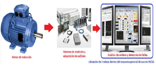
Fig.1 Global scheme for the use of MCSA
It is based on a study and implementation using LabVIEW software platform method based in applying the Fourier Transform for spectral analysis of the feed stream called induction motors MCSA.
2.1 MCSA foundation
For analysis of the effect of the broken bars on the supply current (stator current) of an induction motor we will use the
305
IJCE 2016
general equation linking frequency (f), with the speed of the rotating field (n) and number of pole pairs of the machine (p), being this:
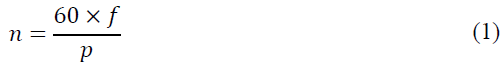
According to Theorem Ferraris, if made them a stator consisting of three coils of phase 120 ° in the circular space a system of three-phase currents balanced, the time lag is 120 °, a rotating magnetic field that surrounds is induced to rotor. This variable magnetic field will induce an electromotive force in the rotor according to the law of induction Faraday force through the same circulation of a current, which in their interaction with the field will generate a torque that will move the rotor. Denoting by n1 speed in r.p.m synchronous rotation, ie the field created by the three-phase stator currents as a function of the frequency f1 of these feed streams and the number of pole pairs 𝑝 of the machine we have:
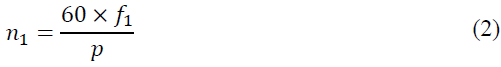
306
IJCE 2016
Suppose the rotor rotating under load at a certain speed n in r.p.m. The speed difference between the field and the rotor  is the relative rotational speed with which the field lines intersect the rotor conductors and under this velocity difference are induced in the rotor winding e.m.f. and currents of a frequency f2 expressing in equation (1).
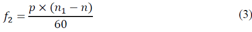
The rotor polyphase currents in turn create a rotary field at a speed , in relation to the rotor in question and in the same direction as the stator field following the inductive sequence which it comes from. It is shown that relative to the stator, the rotor rotates at the speed field as:

That is, it rotates at the synchronous speed, regardless of the rotor’s itself. Fields, stator and rotor remain stationary for one another and could be combined into a single rotating field that ultimately is left as resulting in the machine. It is important to
307
IJCE 2016
note that in any healthy motor the speed of rotation of the rotor currents and fluxes behave or react this with respect to the stator e.m.f. inducing therein the same frequency f1 constant power line. The difference between the synchronous speed and the rotor speed is called slip speed , and is expressed per unit regarding n1 is represented as:
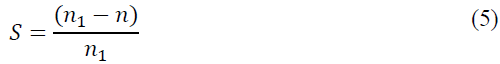
According to equations (3) and (5) can be rewritten expression for the frequency associated with the sliding speed (f2), corresponding to the frequency of the current and e.m.f. induced in the rotor:
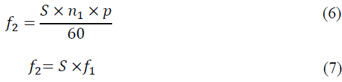
If the engine has broken bars or unbalanced conditions, it creates asymmetry generating an additional magnetic field
308
IJCE 2016
delay, which turns sliding speed, this is Sn1 respect to the rotor [5]. With the presence of this field a stationary observer in the stator windings a rotating field will observe a resultant speed nr defined:

It clearing of (5) the motor speed n in replacing (8) is obtained:

Multiplying both sides of (9) by the number of pairs of poles 𝑝 and considering the expression (1) is obtained:
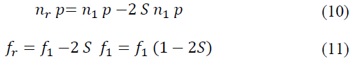
As the rotating magnetic field frequency fr short the stator windings, is induced in them an e.m.f. and hence a current with the same frequency of the rotating field, called fnr, since it corresponds to the frequency of the current through the stator windings as well:
309
IJCE 2016

This implies that under conditions of asymmetry resulting from broken bars in an induction motor, there is the presence of a sideband 2sf1 below the fundamental f1. The effect of broken bars also generates a cyclical variation in the current which results in an oscillatory torque and speed twice the slip frequency [5]. Consequently one sideband 2sf1 appears above the supply frequency f1. In conclusion, it has broken bars in the motor given as components result of currents that are induced in the stator coils and therefore are reflected in the feed stream to the motor frequencies given by (13) around the fundamental frequency f1:

It is important to note that it is normal for an induction motor which don´t have broken their bars present this asymmetry due, for example, an imbalance in the impedances of the windings, but these asymmetries are small comparable to those caused by the effect of the broken bars. That is why the presence of the
310
IJCE 2016
sidebands around the fundamental frequency in an induction motor without failure is normal, but the amplitude of these sidebands are intensified with the broken bars and precisely is the amplitude ratio between the components critical current and these sidebands those considered for diagnosis.
Table I shows the criteria to diagnose broken bars in induction motors using MCSA [6].
Table 1 Fault diagnosis for MCSA
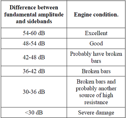
311
IJCE 2016
2.2 Frequency analysis
Fourier transform FT is a mathematical tool used to convert a signal from the time domain to a signal in the frequency domain in order to observe the behavior of a function at a specific time. If it has a signal defined by a function periodic f in the spectrum of frequency discrete, and if is considered a new function g no periodic defined in  , and such that
  in the interval
  . New non-periodic function that results from f is:
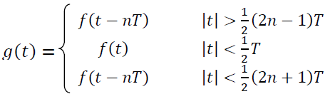
The function f Fourier integral representation is given by the equation expression (14) is:
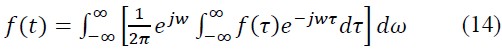
Where j is the imaginary unit, and it must meet two conditions
312
IJCE 2016
sufficient for the existence of equation (14), which is a corrected form of the equation of Dirichlet, and posed as f must:
- be absolutely integrable in , or  is convergent.
- have a number finite of maximum and minimum and be continuous by sections. In addition, equation (14), can be written:

To the expression defined in (15), it is called Fourier transform of f and provides a representation in the domain of the frequency of a function not periodic f[7]. FThas been approached from the format, closer to their use in methods and computational algorithms discrete signal; whose formulation is presented in equation (16).
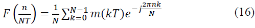
Where n=0,1,2...(N-1) and 𝑁 is the number of samples of the window to be analyzed,Tis the sampling period (inverse of
313
IJCE 2016
the sampling frequency),n is the index of the frequency whose value we want to obtain and m(kT), indicates a sample taken at instant kT(k-th sample) in the area where the images of non-periodic function coincides with the image of the periodic function. The foundation on which the FT is based lies in the comparison of several sine waves and simple cosine with the complex signal analyzed, the more matches a simple wave with the complex signal, the more important is its frequency in determining the original signal. At this point it should be noted that when we analyze a signal frequencies, the information we consider relevant are the frequencies of simple signals with greater amplitude obtained from the decomposition of the original signal [6]. Implement DFT Discrete Fourier transformation on N samples requires approximately N2 complex operations in a time consuming process. For this, the algorithm computationally Fast Fourier Transform (FFT) allowing calculation of DFT in fewer operations, approximately N log2(N) is applied (If N is a power of 2) and therefore operations realize much faster [8] [9].
314
IJCE 2016
2.3 Frequency analysis implemented with LabVIEW
LabVIEW is a graphical programming software created by National Instruments and it has integrated functions for data acquisition, instrument control, measurement analysis and data presentation. The main feature of this software is its ease of use, since it has an extensive library of powerful tools to create relatively complex applications without writing code lines of text. Programs developed with LabVIEW are called Virtual Instruments (VIs) which can be used in turn as building blocks for more complex programs. Each VI consists of two parts: the front panel, which is the interface used to interact with the user when the program is running and the block diagram, which is the program itself and where the icons are placed that interconnect with each other and perform the functions established [10].
Power Expectrum.vi the FFT Power Measurements Waveform tool corresponding to the library Signal Processing shown in Fig. 2 was used to implement the FFT algorithm.
315
IJCE 2016

Fig.2 FFT Power Expectrum.vi
In Fig. 3 and Fig. 4 the front panel of the system and part of the block diagram of the main program where as mentioned above programming is developed and is invisible to the system operator, as this only interacts with the front panel where shown operates controls and receives information.
316
IJCE 2016
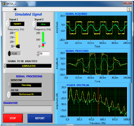
Fig.3 Front panel
Through the control call signal to be analyzed it can choose the signal source to study, with the options: Simulated corresponding to a signal generated by the same system through appropriate controls, Stored in disco corresponding to a signal that has been taken offline and stored in a file, and finally Acquired from, or Acquired from abroad which refers to
317
IJCE 2016
a signal that is online by an acquiring data plate and can be processed at the same time Fig. 5 describes these options.
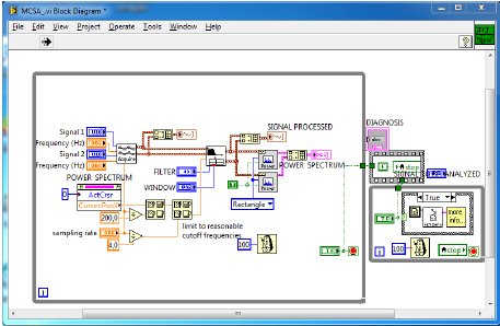
Fig.4 Block diagram
318
IJCE 2016
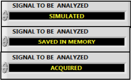
Fig.5 Options control signal to be analyzed
Since our interest is focused on signal analysis, rather than technical data acquisition and considering choosing LabVIEW as a deployment platform, the acquisition and signal conditioning, our tests were carried out with signs stored on disk. Note that the system is able to process signals from the outside once it has the corresponding procuring plate.
3 ANALYSIS AND DISCUSSION
The vibrations in a machinery are directly related with the useful
319
IJCE 2016
life by two ways: a low level of vibrations is an indication that the machine works correctly during a long period of time, while an increase in the level of vibrations report that the machine is heading towards some type of failure, since about 90% of machinery failures are preceded by a change in the vibration feature.
The results are showed after test two induction motors with squirrel cage, one with healthy rotor and the other with broken bars. Table II shows the data of the engines tested which have been provided by Massey Technical Service Laboratories.
Table II Engines tested data.
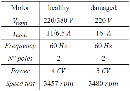
320
IJCE 2016
Fig. 6 and Fig. 7 shows the results of testing a damaged motor rotor
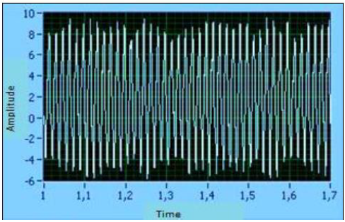
Fig.6 Time response of the motor current damaged
321
IJCE 2016
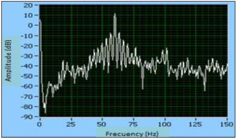
Fig.7 Frequency spectrum of the motor current damaged
Fig. 8 shows the report frequency response in the range of interest and diagnosis of the engine as the view expressed in Table I. They can be observed current frequencies peaks 60 Hz, 63,33 Hz, and 56,67 Hz, corresponding to the fundamental and the sidebands coincide with those expressed in equation (13). The difference between the highest peaks of the sidebands and the fundamental 19,22 db, which means that the engine is in severe damage to the rotor.
322
IJCE 2016
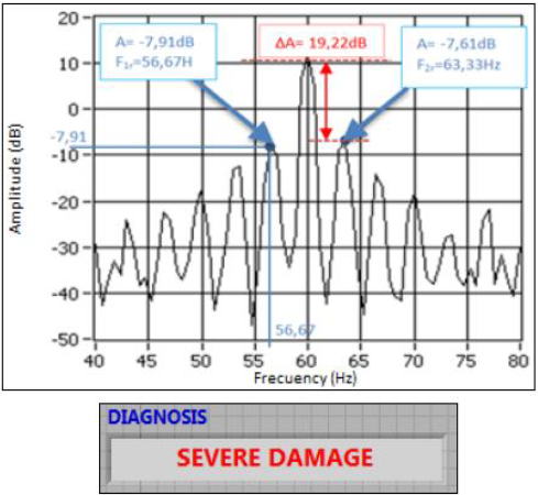
Fig.8 Motor test report damaged
Failures should be detected when they still do not significantly affect the machine so as to perform in this way the corresponding preventive maintenance. Otherwise, the fault would affect significantly the operation of the engine at the moment of its identification, resorting to the model of
323
IJCE 2016
maintenance corrective.
Fig. 9 and Fig. 10 show the results of testing a healthy motor rotor.
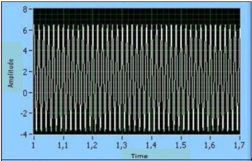
Fig.9 Time response of the current healthy motor
324
IJCE 2016
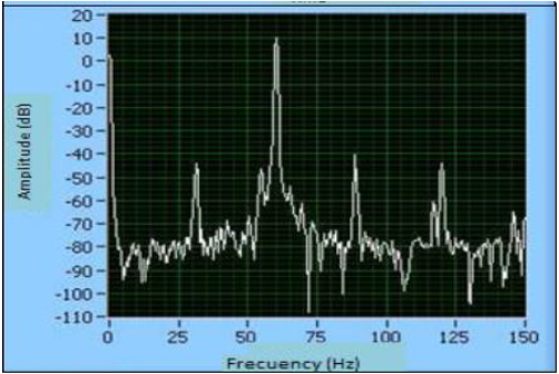
Fig.10 Frequency spectrum of the current healthy motor
Fig. 11 corresponds to the report of the frequency response in the range of interest and diagnosis of the engine as the view expressed in table I.
325
IJCE 2016
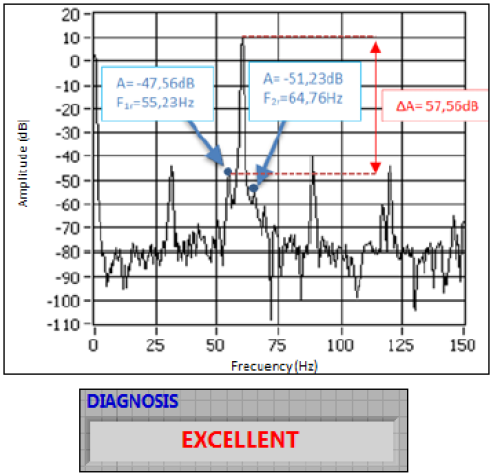
Fig.11 Test report for healthy motorr
Troubleshooting is facilitated with increasing engine load, since the higher the load, the lower the speed, the greater the slip, resulting in greater distance between the fundamental harmonic and sideband and therefore easier to distinguish.
326
IJCE 2016
It is recommended that the fault diagnosis is made with the engine close to the rated load.
The amplitude of the side harmonics is proportional to the degree of fault of cage motor, so the difference in dB between the magnitudes of fundamental and harmonics decrease as more broken rotor bars exist in the cage.
Broken rotor bars on the motor creates two lateral bands on current’s frequency spectrum, located on doubles frequencies of the frequency slide (2sf1) among fundamental frecuency f1.
Analyzing voltage signals in addition to the current, the method can diagnose failures both electrical, and mechanical among which are: broken rotor bars breaking rings rotor shorts the stator coils, rotor eccentricity, bearing failures, among other. The possibility along with the implementation of the signal acquisition stage is presented on the horizon as a continuation of this work in the future.
MCSA requires a frequency analysis, and having digitalized and filtered signals, it must calculate a FDT ( Fourier discrete transform), with the purpose to optimize the computational process, it uses the FFT (Fourier fast transform) which is an algorithm than allow to calculate the FDT faster.
327
IJCE 2016
The Hanning window, generally, is the better way that fit frequency analysis system, like the implemented in the project, due that the system has lineal characteristics and break-off suppressions.
4 CONCLUSIONS
The Motor Current Signal Analysis (MCSA) is one of the most popular used method because for the following reasons. Firstly, it is noninvasive. The stator current can be detected from the terminals without breaking off drive operating. Secondly, it can be measured online therefore makes online detection possible. Thirdly, most of the mechanical and electrical faults can be detected by this method.
MCSA is presented as an excellent alternative online monitoring to diagnose a lot of faults in induction motors becoming a tool to consider in predictive maintenance schemes. It is necessary to stress that for the proper implementation of the MCSA as predictive maintenance tool, is necessary condition the prior knowledge of the state of operation of the engine and its evolution over time. Therefore it is advisable to perform tests on
328
IJCE 2016
the engine periodically in order to determine the evolution of the motor.
This technique can be fairly simply, or complicated, depending on the system available for data collection and evaluation. MCSA technology can be used in conjunction with other technologies, such as motor circuit analysis, in order to provide a complete overview of motor system health.
Using LabVIEW technology allows the implementation to be user friendly and facilitate the collection, processing, data storage and the ability to generate reports and statistics in a simple way.
REFERENCES
1. W. Thomson, M. Fenger, Current Signature Analysis to detect induction motor faults, IEEE Industry Applications Magazine, Vol.7, No.4, 2001, pp. 26-34.
2. D. Raheja, J. Llinas, R. Nagi, Data fusion: Data mining based on architecture for condition based maintenance, International Journal of Production Research, Vol.44, No.14, 2006, pp. 2869-2887.
329
IJCE 2016
3. R. Puche Panadero, M. Pineda Sanchez, et al., Improved Resolution of the MCSA Method Via Hilbert Transform, Enabling the Diagnosis of Rotor Asymmetries at Very Low Slip, IEEE Transactions on Energy Conversion, Vol.24, No.1, 2009, pp. 52-59.
4. C. Verucchi, G. Acosta, Fault Detection and Diagnosis Techniques in Induction Electrical Machines, IEEE Latin American Transactions, Vol.24, No.1, 2007, pp. 41-49.
5. N. Ngote, S. Guedira, M. Cherkaoui, A new approach to diagnose induction motor defects based onthe combination of the TSA method and MCSA technique, Proceedings of WSEAS Transactions on Signal Processing, Vol.8, No.3, 2012, pp.77-86.
6. Massey Technical Service, EQUIPMENTHEALTH Motor Current Signature Analysis, 2001, http://equipmenthealth.com/mcsa.htm
7. J. Bobadilla, P. Gomez, J. Bernal,. La Transformada de Fourier: Una visión pedagógica, Departamento de Informática Aplicada, Escuela Universitaria de Informática de Madrid, 2001, pp. 43-74.
8. G. James, Matemáticas Avanzadas para Ingeniería, Prentice Hall,
330
IJCE 2016
2002.
9. H.Kwakernaak, R. Sivan, Modern Signals and Systems, Prentice Hall, 2000.
10. V. Lajara, S. Pelegrí, LabVIEW: Entorno gráfico de programación, Alfaomega, 2006.
11. W. Thomson, R. Gilmore, Motor Current Signature Analysis to Detect Faults in Induction Motor Drives-Fundamentals, Data Interpretation, and Industrial Case Histories, Proceedings of 32nd Turbomachinery Symposium, 2003, pp. 145-156.
12. N. Mehala, R. Dahiya, Motor Current Signature Analysis and its Applications in Induction Motor Fault Diagnosis, International Journal of Systems applications, Engineering & Development, Vol.2, No.1, 2007, pp. 29-35.
13. M. Castelli, J. Fossati, M. Andrade, New methodology to faults detection in induction motors via MCSA, Transmission and Distribution Conference and Exposition: Latin America, 2008 IEEE/PES, August 2008,pp. 1-6
331
IJCE 2016
14. A. Singhal, M. Khandekar, Bearing Fault Detection in Induction Motor Using Motor Current Signature Analysis, International Journal of Advanced Research in Electrical, Electronics and Instrumentation Engineering Vol.2, No.7, July 2013, pp. 3258-3264
15. S. Haus, H. Mikat, M. Nowara, et al, Fault Detection based on MCSA for a 400Hz Asynchronous Motor for Airborne Applications, International Journal of Prognostics and Health Management, 2013
332
ICERI 2016
EDUCATIONAL TECHNOLOGY INTERVENTION FOR THE
DEVELOPMENT OF ADVANCED CALCULUS APPLICATIONS Descargar pdf
Alicia Tinnirello, Eduardo Gago, Mónica Dádamo
Universidad Tecnológica Nacional (ARGENTINA)
Abstract. Students of Engineering often find a great amount of difficulties in subjects where the practical application of the theoretical concepts is essential. This paper describes the various innovative experiences implemented in the classrooms of advanced calculus, part of the 3rd course of the engineering studies, where mediation between the content of the subject and expected responses from the student group, was given through the gradual incorporation, in workshops classes, of different technological applications (Mathematica, LabVIEW, Comsol) and the use of virtual learning platforms. Over the years, the implementation of methodological strategies had each own and distinct characteristics in terms of the activities and results
333
ICERI 2016
achieved, in the sense of the contributions made to the training in engineering. This strategy is supported on the technique of different projects, and has been carried out for six years. Students have showed a significant interest and motivation for this activity and their opinions in respect to the use of these practices have been absolutely positive, thanks to several factors such as: flexible schedules and tutorials, the coordination between seminars and theoretical learning, the set of problems and practical cases proposed, the organization of the seminars and a fluent communication between students and teacher. Educational interventions that use technological applications available to explore concepts of modeling, estimation of parameters, numerical simulation and analysis of cases in search of better understanding of concepts and procedures have been developed. On the other hand, there was an emphasis on the results achieved by the students after using technological applications to validate, verify properties, classify or perform calculations that are complicated in the contents of the subject (complex variable, Laplace transform, Series and Fourier Transforms). Different innovative educational experiences, which the Department has implemented in recent years in the teaching
334
ICERI 2016
of the advanced calculus, have allowed revealing the
change experienced by teaching of thinking about the construction of the technological scientific
knowledge, within the framework of the new epistemological view of the science. On the one hand,
traditional techniques that allow observing the analysis of causality are used. On the other hand, by
using computer programs oriented to complex systems and control, employing the algebra of blocks
and arrows to feedback, models are obtained starting from their constitute and structural relations,
which allow to transform such models in ordinary differential equations systems and at the same time,
use certain analysis techniques directly in their flow sheets.
This approach includes the concepts of feedback and ports, as well as the vision that emerges from
the paradigm of OOP (Object Oriented Programing), to create databases and to be eligible for various
resolution techniques, as also to incorporate those concepts that allow solving systems of more than
one degree of freedom, non-linear systems, with multiple inputs and outputs. Through this way there is
a break to the model of only one thought and the future engineer is prepared to handling a complexity
that today is unavoidable.
335
ICERI 2016
Keywords: multidisciplinary problems, undergraduate education, virtual instruments, signal processing.
1 INTRODUCTION
In search of a multidisciplinary training, the incorporation of technology in higher education allows
significant changes in the teaching and learning process, that impact on engineering careers,
especially in the area of Mathematics. Specific software and computational tools insertions, which are
increasingly powerful, allow making the modifications needed to achieve this purpose.
With the objective to carry out these changes, we need to align the university curricula not only to the
new work methods that allow intellectual development stimulation, but also have a tendency to a
multidisciplinary approach. The goal is not only to teach and learn only mathematics, is also doing it by
facing them with the stimulation of real cases and simple systems that lead the student to have a look
at real situations.
336
ICERI 2016
It is noteworthy that students are encouraged when they leave aside traditional forms of paradigmtype
problem solving, and when they are imposed to a significant and reflexive learning dynamic that
involves engineering situations which ignore idealism and are related to the ones to be carried out in
practice. Sometimes it is observed that the students do not follow abstract and general processes, or
find it difficult to adapt to them. This is why the trend in contemporary education needs the
implementation of a system that places the student in centred processes that identify him as an active
and reflective learning subject.
Project based learning has proved to be a suitable method to demonstrate the need of mathematics in
professional engineering. Students are confronted, complementary to their regular courses, with
problems that are of a multidisciplinary nature and demand a certain degree of mathematical
proficiency.
The curricula of the Mechanical Engineering programs at our university include Advance Calculus at
the third year of the engineering studies; the authors’ experience is that students increase their
interest and their appreciation for the contents
337
ICERI 2016
when they are involved by learning in an applied way.
In the introduction to the modeling of physical and engineering systems and the design of control
systems, information technologies converge with the advanced elements of the mathematical
calculation. The systemic and analytical paradigms of unsupported philosophical roots overlap giving
rise to a new pedagogical and didactic proposals. The primary focus of the analysis proposed treats
the concept of feedback or feedback form related with mathematics associated with the study of
invariant linear systems over time (SLI).
It seeks to introduce the concept of feedback in an early stage in the engineering curriculum, and to
show the compatibility between the treatment of systems in a traditional way - by means of differential
equations – obtained by using computer programs, to complex systems and control - using the
algebra of blocks and feedback arrows.
2 METHODOLOGICAL APPROACH
When systems and simple phenomena are studied, it can be considered that an efficient management of the object in study
338
ICERI 2016
is linked in direct way with the understanding of the topic. When complex
systems are studied, the relationship between the operational knowledge and the explanatory and
justification areas is potentially more diffuse.
An example of this is observed in the study of the SLI, in which through its calculation the learning of
the following themes is jointly introduced: Laplace transform, Fourier transform, transfer matrix,
convolution, and so on.
One of the not desired outcomes of this conjunction of elements owned to SLI is considered to the
respective transfer function (FT) as obtained by means of the Laplace transform, when the input is the
unit impulse.
If we focus on the properties inherent to the linear system, highlighting that the FT is characterized by
the linearity of the differential operator, that describes the model, the constant coefficients described a
SLI system, so that it is selected the "side" that corresponds to the system, separating it from the input
function.
With a SLI of the obtained solutions, an analytical approach by means of differential equations can link
with the ones obtained from an systemic approach, with simulation systems, by means
339
ICERI 2016
of diagrams of
blocks and ties of feedback, and not as technical unconnected between itself.
This alternative way to obtain the solutions of differential equations is motivated by:
• Current control systems (Basic, type PID) use feedback in its intrinsic form and are of massive
diffusion within the industry.
• When the system is more complex, there is greater incidence of the computational component
in mathematics and the computer science advances toward the paradigm of OOP, which we
can associate with the algebra of blocks and blocks in an objective manner.
• The concept of feedback is a recent addition to the field of science and technology, born in the
Second World War and the interdisciplinary wedge; both aspects make difficult their
incorporation into the curriculum of basic education.
• Cybernetic and systemic the "feedback", although complements the analytical engineering
vision, it resists to be boxed in the reductionism of the classic physical [1].
To show the interaction of disciplines that arises in the professional practice in the different
environments of work, and approach students to real problems, not only the conventional
340
ICERI 2016
ones, but
also those of recent development with different techniques of analysis and mathematical models
involved, a systemic approach is presented, - key component in the professional software for modeling
and simulation-, providing new strategies in the study, through the use of virtual platforms for
modelling and simulation of dynamic systems.
In the undergraduate degree in engineering, feedback is treated in mathematical studies of SLI
systems, and usually associated with programs that implement it for the treatment of complex
systems, with little or no mention of the systemic approach.
In this presentation the concept of feedback shown efficient and compatible management of
mechanics Newtonian. Although the form of relating it shows a rupture with the thoroughness
traditional of the analytical approach, is consistent with the paradigm of the complexity, where the
reasoning analog, added to it effectiveness verifiable, is considered valid.
In a simple way, we mention the systemic approach in early stages, which is of scarce academic
treatment currently and of intensive use in the engineering professional career.
341
ICERI 2016
3 LEARNING SPACE
The Computational and Multidisciplinary Laboratory is a virtual working place in which engineering
students developed intensive activities, using appropriate tools, adding to the process of learning
inputs, systems, controls of mechanisms, tools technology, and so on.; that generate outputs in areas
of students genuine interest . In this space, theoretical and practical activities are organized, where
students develop technical applications, following the subjects developed in class, connecting subjects
between others different disciplines of the same level or of different levels.
The selection of the project, in this case, is the design of virtual instruments (VI) for the study of
systems, not only in the time domain, but also on frequency domain, applying Laplace transform as a
result of the interaction with teachers from the upper cycle of the engineering course.
Professional environments for the simulation of physical or industrial systems (Simulink, Lab-View,
XCos) are used as interface with the user a graphic mode, characterized by block diagrams and their
interaction, incorporating the feedback loop at this last
342
ICERI 2016
aspect.
This possibility not only gives place to the analysis in different conditions but also allows observing
instant to instant the transition between states, which contributes considerably in the understanding of
topics associated to dynamic issues. This methodology has acquired special relevance since it is
essential part of any control system.
4 PRELIMINARY CONCEPTS
In order to build a meaningful learning, both the basics of Laplace's transform and its application to the
resolution of systems using differential equations as an introduction to the algebra of blocks and
rudimentary knowledge of programming in the graphic language, are needed (in this work, LabVIEW).
It requires also a family management of the Fourier transform and the analysis in the time and
frequency domain. These concepts will give the student a satisfactory view of the current state of the
science and technology development linked to the continuous SLI, with the exception of recent
systemic studies, exceeding the objectives of advanced basic training.
343
ICERI 2016
It is intended to further the vision of the analytical approach - present in the classical physics- linking it
with the systemic approach, - key component in the professional software for modeling and simulationproviding
new strategies in the study, through the use of virtual platforms for modelling and simulation
of dynamic systems.
A second-order system is one whose dynamic behavior is represented by the second-order differential
equation in the analysis of the simple dynamic systems such us a mass-spring system (M_S) or an
electrical system R-L-C: In these cases, it is easy to get the model through an Ordinary Differential
Equation (EDO) raising its constitutive and structural relations Fig. 1.
Ordinary Differential Equation (EDO) raising its constitutive and structural relations Fig. 1.
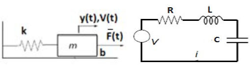
Fig.1 Dynamic systems
344
ICERI 2016
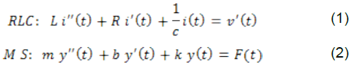
An 'order n EDO' can be rewritten as 'n EDOs order 1 system', named States Equations. On this way,
it is defined 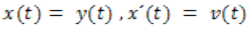 for the equation (1) the system is
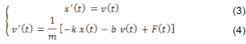
Where  are called state variables.
In circuit RCL, defining
are called state variables.
In circuit RCL, defining 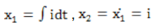 , we get the system:
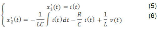
Where 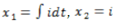 is the state variable
Even though the continuous systems are represented through differential equations models, it is very difficult to obtain the
345
ICERI 2016
right equations directly when the model grows up in complexity: The equations
systems cannot be coupled to get complex models from simple models, to get the EDO, from the
consecutive and structural relations, it is necessary algebraic effort and obtained models have not got
visual similarities with the originals schedules.
Applying Laplace transform to the response system function and to the entrance function we defined
the transfer function useful to characterize the input-output SLI systems. It can be represented by
blocks diagrams describing the system.
5 DEVELOPMENT OF THE APPLICATIONS
5.1 Respond of second-order systems to various inputs
The second-order system has the characteristic parameters: the steady state gain, the damping coefficient and the natural period or the inverse natural frequency. The second-order transfer function has no zero, but has two poles located at s=r1 and s=r2, where r1 and r2 are the two roots of the denominator
346
ICERI 2016
quadratic [2]. The students work analyzing the different possibilities for the response, using the software LabVIEW, of simple and practically intuitive way, is develops the structure graphic that models the system oriented to the analysis of the nature of these roots [3].
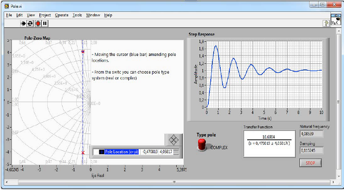
Fig.2 Underdamped response
These diagrams allow us to analyze all the states that adopt the
347
ICERI 2016
system as we modify the parameters
of the system under study. Fig. 2 shows the front panel of a VI that is associated with the location of
the roots of a system of 2nd order and its effect on the response to input step.
The application allows moving the pole to the desired locations, and emits the place of roots that
shows the locations of the poles of the closed-loop (feedback), the natural frequency and the damping
coefficient and response to the step of the system corresponding to these locations. Alternatively, you
can specify the real and imaginary components directly in the legend below the graph. Are evident
what this application gives to the student in order to show the relationship between the displayed
parameters and their influence on the time response. At the same time can be seen relate these
margins of stability with the time response of the system to an step or ramp input, swings, steady-state
errors, and so on.
In the figures can be observed, the relationship of the response transient with the location of poles
being this each time more damped as them poles is located in places real negative coming to be
critically damped when poles are equal and real. When poles are real and equal the system is
overdamped and
348
ICERI 2016
implies there are no oscillations.
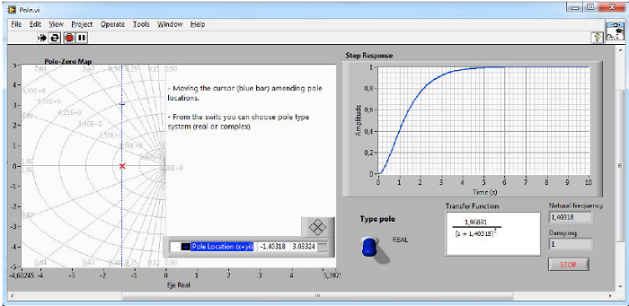
Fig.3 Critically damped system
The relationship of the oscillation of the transient response can observe as the complex conjugate
poles are moving towards higher values of imaginary component and less than real component, to the
extent of becoming totally oscillatory for pure imaginary poles.
349
ICERI 2016
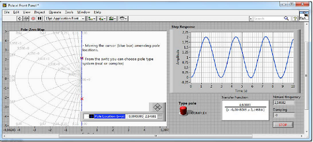
Fig.4 Complex conjugate poles
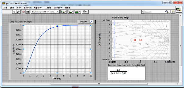
Fig.5 Overdamped Systems
350
ICERI 2016
The Fig. 4 shows complex conjugate poles with little damping response with more oscillations, in this
case the real negative part of poles is small. The system is called critically stable and the response
has sustained oscillations.
The sliding controls allow to modify the system parameters and to observe at the same time its
evolution in the graphic, facilitating the teaching and complementing the explanation of themes as:
systems mathematical modeling, limitations of operating in the domain of time with differential
equations, giving rise to a new domain using the Laplace transform and other related topics.
The application allows to move the poles and to locate the place of roots showing both, the locations
of closed loop poles and the natural frequency, damping coefficient and response to the step of the
system. Alternatively, we can specify the real and imaginary components directly in the legend below
the graph, the advantages that this graphs provides for teaching are evident, showing the relationship
between the parameters displayed and its influence in the temporary response.
351
ICERI 2016
5.2 Frequency Respond of second-order systems: Stability
The frequency respond methods provide a graphical tool for the design and analysis of a system. The different graphics present the front panel of a VI that shows the effect of the action of different types of controlled systems with different types of controllers and their analysis in the time and frequency domain. Within the VI block diagram systems of any nature (electrical, chemical, mechanical, i.e.) can be represented, whose behavior can be described by differential equations and be represented in the form of using the Laplace transform transfer function [4] [5].
352
ICERI 2016
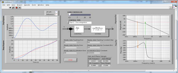
Fig.6 System with wide range of phase and gain, oscillatory and slow response
By the observation of the effect of different types of system’s drivers in the analysis and errors calculation in stationary state, and the response of the step and ramp input at the same time, it is easy to display as such changes affect the frequency response by means of bode diagrams and the corresponding gain and phase margins [6].This is very useful as it allows the student to demonstrate graphically how the effects of a modification in a controlled system manifest themselves differently depending on the domain in which they are being analyzed, whether it’s the time response and/or the frequency
353
ICERI 2016
response, allowing the student to relate the concepts with more clarity. Gain and phase margins allow us to analyze the stability of a system negative feedback though the system in open loop frequency response.
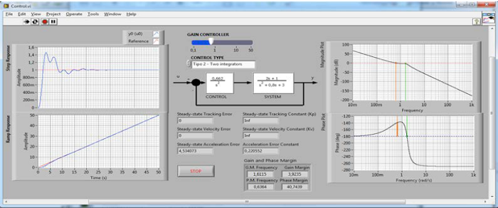
Fig.7 System with less margin of phase and gain and less oscillatory response
354
ICERI 2016
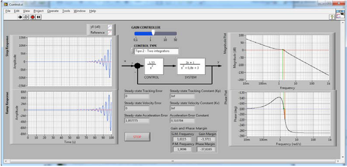
Fig.8 System unstable
From Fig. 6, 7 and 8, we can observe that the margin of profit is positive and the system is stable if the magnitude, to the crossing of phase of-180 °, is negative (in db). I.e., the axis 0 db, will be negative and an unstable system. The phase margin is positive and the system is stable if the phase is greater than 180 ° at the junction of 0 dB gain. I.e., the margin of phase is measured above the shaft-180 °. If the margin of phase is measured down the shaft-180 °, the margin of phase is negative, and the system is unstable.
355
ICERI 2016
6 CONCLUSION
The design and interpretation of these virtual instruments will allow students to observe the effect of different types of drivers in the systems, the analysis and calculation of the errors in stationary state and the response to the entry step and ramp. At the same time this will allow them to see how such changes affect the frequency response by means of Bode diagrams and the corresponding gain and phase margins. The latter is very useful, since it allows the teacher to show in a didactic way and in real time how the effects of the same modification in a controlled system manifests itself differently depending on the domain in which they are analyzed; in the time response and/or frequency response, making it clear to the student how to relate these concepts. The proposed methodology favors the student’s interpretation of issues associated with dynamic conditions, its relationship with the differential equation which describes the system, and its corresponding transfer function obtained through the Laplace transform, while bringing them a software simulation tool similar to the ones they will find in the field of their professional life.
356
ICERI 2016
ACKNOWLEDGEMENTS
The authors would like to express their recognition to the student Lucas D’Alessandro for his performance during the development of his project work.
REFERENCES
1. K. Astrom, R. Murray, “Feedback Systems: An Introduction for Scientists and Engineers”,
Princeton University Press, pp. 201-226, 2009.
2. A. Batatunde, A. Ogunnaike, W. Harmon Ray, “Process Dynamics, Modeling, and Control”
Oxford University Press, pp. 430-459, 1994.
3. V. Lajara, S. Pelegrí, “LabVIEW: Entorno grafico de programación”, Edit. Alfaomega, Madrid,
pp. 175-185, 2006.
4. G. James, et al, “Matemáticas avanzadas para ingeniería”, Edit. Prentice HALL, México, pp.
178-202, 2002.
5. K. Ogata, “Ingeniería de control moderna”, Edit. Pearson, Madrid,
357
ICERI 2016
México, pp. 178-202, 2010.
6. Y. Lin, “Grey Systems. Theory and Application”. Edit. Springer-Verlag, Berlin, pp. 475-479,
2011.
358
ICERI 2016
VIRTUAL INSTRUMENTS INTEGRATING MATHEMATICAL
MODELING FOR ENGINEERING EDUCATION Descargar pdf
Alicia Tinnirello, Eduardo Gago, Lucas D’Alessandro, Mónica Dádamo
Universidad Tecnológica Nacional (ARGENTINA)
Abstract. Engineering students need to learn how to formulate mathematical models of physical situations, how to obtain useful solutions to the model equations, and how to correctly interpret and present the results. We want to introduce our engineering students to problem-solving with modern engineering tools, such as LabVIEW, applied to more realistic problems. The use of technology in undergraduate engineering curriculum is ongoing matters of interest. It is essential that students do not lose sight of the physical phenomena being modeled, the assumptions behind the mathematical models used, or the need to verify and validate the computational methods applied to the problem. Similar concerns have been raised regarding the use of process
359
ICERI 2016
simulation software to carry out signal processing
systems, and successful implementation of these advanced computer tools may require a re-focusing
of course objectives and skills taught, and a re-structuring of the course curriculum. The course on
advanced calculus level undergraduate try to show industrial applications and in this case we focused
in motor induction functioning. This paper show the interest focus only on signal analysis, rather than
technical data acquisition, particularly in fault detection by broken bars in squirrel cage induction
motors and the task of signal analysis and subsequent diagnosis, leaving aside the proper signal
acquisition implemented using LabVIEW software platform, based on the method of applying the
Fourier Transform for spectral analysis of the feed stream. Since our interest is focused, considering
choosing LabVIEW as a deployment platform is intentional because it facilitates the acquisition and
signal conditioning, the tests were carried out with signals stored provided by Massey Technical
Service Laboratory.
Project development in a teaching process is to work in a multidisciplinary form similar to future
professional work, in this way the teachers look forward subjects of student’s interest. In
360
ICERI 2016
this case,
simulated online condition-based maintenance strategies are presented. Current motor signature
analysis (MCSA) is the online analysis of its current, to detect faults in a three-phase induction motor
drive while it is still operational, and in service, so that the students follow this method in order to
monitor several faults on diagnosis induction motors in a virtual laboratory. LabVIEW allows an userfriendly
implementation and facilitates collection, processing, data storage and report generations and
statistics in a simple way.
This methodology allows students to increase their abilities because there is an articulation of the
content of mathematics that favors the interdisciplinary perspective using and discovering
mathematical concepts through the proposal of real-life situations. It’s put the emphasis on
methodological change versus traditional teaching, so as to acquire a heuristic aspect that highlights
the mathematics’ epistemology and it give a new meaning to the evaluation processes.
Keywords: multidisciplinary problems, undergraduate education, virtual instruments, signal processing.
361
ICERI 2016
1 INTRODUCTION
The evolution of technology, along with sophisticated communication systems and economy, the latter
currently undergoing a serious crisis at global level, require modern society to be absolutely subjected
to these profound changes.
Education systems in higher education are not exempt from this influence and are permeable to these
changes that cause the need to: review and adapt academic management, reorganizations, changes
in curricula, and consequently changes in the processes that regulate teaching and learning in the
universities.
In a changing and dynamic society, we cannot attempt to introduce students to the contents in a
formalized and abstract way. Moreover, the ability to master contents should not be as important as
the ability to know how to search for them, evaluate them, and adapt them to the specific requirements
that may be needed at a particular time. Under this premise, one should not ignore that to function in the society of the future, students should possess new capabilities, such as adaptability to an
environment that is rapidly changing; Teamwork; apply
362
ICERI 2016
creative and original proposals to solve
problems; ability to learn; unlearn and relearn; learn how to make decisions and be independent; apply
the methods of abstract thought; being able to identify problems and find solutions [1].
In addition, the advent of computer media, so attractive and friendly to students, not only because of
its wide possibilities of work, but the familiarity with which students operate with them, have impacted
heavily on education. All these issues translate into challenges posed by the need to maintain
horizontal and vertical connections with the subjects of the curriculum. Students demonstrate a lack of
motivation being experienced in different subjects of the Basic Cycle, either because their find its
content disjointed and abstract or, they cannot relate it with their chosen studies [2].
Simulation and modeling of problematic situations help to conceptualize and visualize calculation
topics involved in the development of subjects of the upper cycle of their studies or in their
professional life, and facilitate learning modes.
The didactic proposals presented allow explaining subjects in Higher Mathematics through means of
research and application of analytical, qualitative, graphical and numerical methods, in
363
ICERI 2016
order to study various mathematical models that describe representative phenomena of physical systems that characterize engineering processes.
2 METHODOLOGY
The background problem on how to provide education resides in creating the conditions so the
knowledge schemes that students built evolve in a specific direction. The students need to have
enough prior knowledge to address the contents proposed, in order to establish more complex and
rich relationships between them, so as to increase the significance of their learning [2].
At the beginning it is suitable to help the student to remember, reorder or assimilate the previous
necessary knowledge related with the proposed content, so as to deal successfully with the
programmed learning, designing cognitive bridges between the new content proposed and the
structure of knowledge that the student already have (previous organizers). Therefore, appropriate
strategies are developed to place students in situations of favorable learning. This involves an intense
activity
364
ICERI 2016
from the learner and a real commitment from the teacher in what refers to the directionality,
coordination and pedagogical help.
In such sense, an integrated will be developed: theoretical-practical and theoretical-technological, in
an attempt to have a different experience based on: dialogue, convergence of criteria and active
participation of students.
To follow the evolution of their mathematical thinking is necessary to awaken the interest of student in
applications and induce them to form notions and to discover by themselves the mathematical
relations, trying not to impose a single way of thinking, taking advantage of the originality of their
creative spectrum and new points of view.
As long as the student is allowed to relate each piece of knowledge to incorporate with the previous
knowledge already acquired, learning will be more meaningful and functional. Relevant and properly
sequenced questions, so as to guide the student’s line of thought through reasoning that allow them to
reach certain conclusions -convergent thinking-, will make its exposure more dynamic and
participatory [1] [2].
The teacher will act as a learning facilitator, guiding with
365
ICERI 2016
questions, presenting situations, pointing out
errors and avoiding resolving what the student can resolve on their own. The situations raised will be
simpler in a first stage increasing gradually its level of complexity.
Simulation platforms have a fundamental role, both in what refers to teaching mathematics, to its
applications in engineering.
To carry out the proposal of this new vision of education, which contributes in making contact with
activities related to the discipline, we count with a basic science computer laboratory where students
develop experimental classes; to generate a virtual work environment, where they perform activities in
autonomously, with the collaboration teachers trained in the teaching methodology.
3 PRESENTATION OF DIFFERENT PROPOSALS
The educational activities proposed consist of a theoretical investigation of the subject to be developed by students under the supervision of teachers, to then develop an analogy with the physical parameters of the subject under study and finally, with the gathered information, solve the proposed problem situation
366
ICERI 2016
with technological resources.
3.1 Case No. 1: Signal response of 2nd order system
In this case, the methodology of presenting the mathematical content is based on the search of
models that simulate the situation that we require to formulate or technical situation in mathematical
terms. This is why a simplified situation is presented by translating the situation in mathematical
language, creating the model for classroom work.
Considering an RLC circuit formed by a resistor 160 ohms, a capacitor 10-4 F and an inductance of 1
H serially connected to a voltage source 20 V. Before closing the switch at time t = 0, both the charge
and the resulting current is zero. For determining the charge on the capacitor and the resulting current
in the circuit students propose guiding questions to investigate the system [3]:
− What is the system solution?
− What does each term in the solution represent?
− What are the characteristics of the system?
− What is the electrical and power curves burden the system
367
ICERI 2016
output?
− What is the maximum response system output?
Students determine that the transfer function for the second order load system presented has the form
of equation. (1)
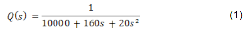
According to the data supplied they obtain temporary solution functions for loading and they analyze the current system:
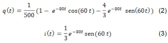
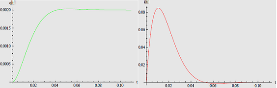
Fig.1 Charge and current in the circuit
368
ICERI 2016
The maximum load on the system is 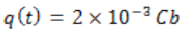 , while the current flowing through the circuit
after a short time is zero
Students analyzed the system behavior using the LabVIEW platform, as shown in Fig. 2.
, while the current flowing through the circuit
after a short time is zero
Students analyzed the system behavior using the LabVIEW platform, as shown in Fig. 2.
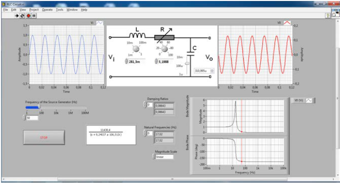
Fig.2 Circuit behavior report
369
ICERI 2016
3.2 Case No. 2: Frequency analysis of electrical signals for detecting faults in induction motors
In this case study it is intended that students perform the analysis and implementation of an alternative
way of detecting and diagnosing faults when a rupture of the bars of the squirrel cage of induction
motors is produced by the spectral analysis of the feed stream known as MCSA (Motor Current
Signature Analysis).
The proposal aims to create a system of signal analysis and fault diagnosis algorithms based on
spectral analysis of currents (MCSA) that is easy to use and adaptable to signals with little prior
conditioning.
Aiming for reliable system, with ease of implementation, an user-friendly interface with students,
scalability and resources optimization that allows the acquisition of signals of multiple forms found in
the industry, with translators that are available in the market with little external conditioning, the
students’ work in the lab is implemented using LabVIEW programming platform created by National
Instrument.
3.2.1 Students Research
370
ICERI 2016
Students will analyze a system to detect failures due to the bars that break in the squirrel cage
induction motor, and specifically, they will perform a task that involves analyzing the signal with the
frequency of the electrical currents in the engine to later to make a diagnosis leaving aside the
acquisition of the signal itself.
Students will study and implement using LabVIEW programming platform application based on the
Fourier Transform method for spectral analysis of the supply current of induction motors with MCSA
technique [4].
We request students to research the theoretical guidelines needed to analyze the operation of two
induction motors, to later determine which engine have the squirrel cage bars in good condition and
which motor has the damaged one. For this purpose the students fill in a report that consists of two
parts.
3.2.2 Theoretical knowlegde
For the analysis of the effect of the broken bars on the supply current (stator current) of an induction motor students have the general equation linking frequency (f), with the speed of the rotating field (n) and the number of pair’s pole of the machine
371
ICERI 2016
(p), being this:
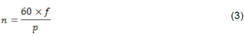
Students use the Theorem of Ferraris, which states that if the stator comprises three coils out of phase 120º in space, are being made to circulate a system of three-phase balanced currents, which time lag is also 120º, a rotating magnetic field is induced to surround the rotor. This variable magnetic field will induce an electromotive force in the rotor, which according to the law of induction of Faraday forces itself through the same current circulation, which in its interaction with the field, set the rotor in motion. If n1 speed synchronous rotation in r.p.m., i.e. the speed of the field created by the three-phase stator currents as a function of the frequency f1 of these feed streams and the number of pole pairs of the machine we have:
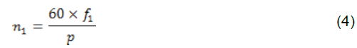
As the rotor rotates under load at a certain speed n in r.p.m., the
372
ICERI 2016
speed difference between the field and the rotor (n1-n) is the relative rotational speed with which the field lines intersect the rotor conductors, and under these speeds differences are induced in the rotor winding f.e.m. and currents of the frequency f2, as expressed in the equation (3):
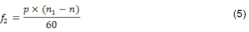
The rotor polyphaser currents in turn create a rotary field speed (n1-n), with respect to the rotor, in question and in the same direction as the stator field following the inductive sequence which they proceed from. It is shown that relative to the stator the rotor rotates at the speed field as:

That is to say, at the synchronous speed, regardless of the rotor itself. Fields, stator and rotor remain stationary from one another and could be combined into a single rotating field that ultimately it is left as resulting in the machine. It is important to note that in any healthy motor whatever the speed of rotation of
373
ICERI 2016
the rotor is, currents and flows behave or react with respect to the stator f.e.m. inducing
therein the same constant frequency f1 than the power line.
The difference between the synchronous speed and the rotor speed is called slip speed (n1-n), and
expressed per unit regarding is represented as:
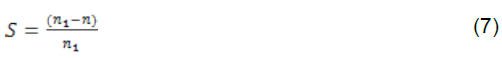
From equations (5) and (7), equations are obtained:

If the engine has broken bars unbalance conditions or asymmetry are created, which generate an additional magnetic field with delay, which turns at sliding velocity. With the presence of this field a stationary observer in the stator windings will observe a rotating field at a resultant velocity which defines the equation (10):
374
ICERI 2016

From equation (7) and by replacing in (10) is obtained:

Multiplying both sides of (11) by the number of pole pair’s p and considering the expression (3) It is obtained:
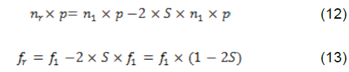
As the rotating magnetic field frequency short the stator windings, It is induced in them an f.e.m. and hence a current with the same frequency fr of the rotating field, called f1r, since it corresponds to the frequency of the current that circulates through the stator windings:

This implies that under conditions of asymmetry, as a consequence of the rupture of the bars in an induction motor,
375
ICERI 2016
there is the presence of a sideband s2f1 below the fundamental f1.
By effect of the broken bars a cyclical variation in the current is also generated which results in an
oscillatory torque and oscillatory speed twice of the slip frequency. [5]
The broken bars in an engine determine currents components that are induced in the stator coils and
therefore are reflected in the stream feed of the motor, frequencies given by (13) around the
fundamental frequency f1:

Table I shows the troubleshoot criteria for broken bars in induction motors using MCSA
376
ICERI 2016
Table 1 Fault diagnosis MCSA
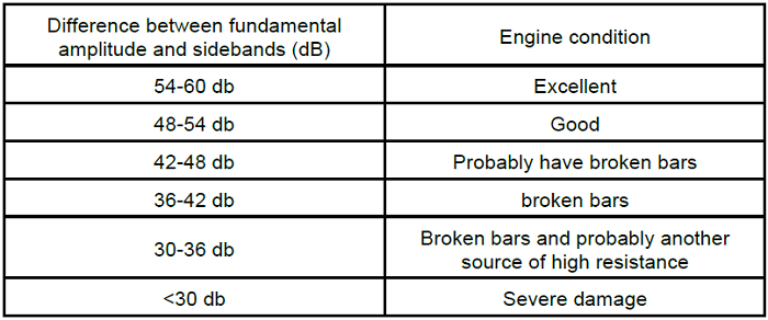
Fourier transform (FT) is a mathematical tool used to convert a signal from the time domain to a signal in the frequency domain, in order to observe the behavior of a function at a specific time. The FT is studied from the format of a discrete signal, closer to its use in methods and computational algorithms; whose formulation is presented in the equation (15). [1]

377
ICERI 2016
Where N is the number of samples of the window to be analyzed, T is the sampling period, n is the
index of the frequency whose value we want to obtain and m(kT) indicates the sample taken at an
instant kT (k-th sample) of the window.
The foundation on which the FT is based lies in the comparison of several sine waves and simple
cosine with the complex signal analyzed, the more a simple wave matches with the complex signal,
the more important is its frequency in determining the original signal. At this point it should be noted
that when a signal frequency is analyzed, the information considered relevant are the frequencies of
simple signals with higher amplitude obtained from the decomposition of the original signal [6] [7].
Implement DTF Discrete Fourier Transformation on N samples requires about N2 complex operations
in a time consuming process. For this, computationally, the algorithm Fast Fourier Transform (FFT) is
applied, which allows the calculation of DTF in fewer operations, approximately N log2 (N) (if N is a
power of 2) operations, and therefore in much faster way [1].
378
ICERI 2016
4 OPERATION ANALYSIS
For the implementation of the algorithm FFT, Students use the LabVIEW tool: FFT Power Expectrum.vi Waveform Measurements, corresponding to the Signal Processing library. In Fig. 3, the front panel of the system is observed, and in Fig. 4 the main program block diagram provided in the report done by students [8].
379
ICERI 2016
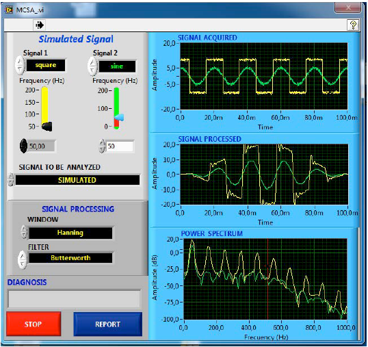
Fig.3 Front panel
380
ICERI 2016
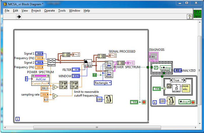
Fig.4 Block Graph
Since the control called “signal to be analyzed” can choose the signal source to study, with the options; “simulated” corresponding to a signal generated by the same system through appropriate controls, “signal stored on disk” this being a signal that has been taken offline and stored in a file, or finally
381
ICERI 2016
“signal acquired externally” referencing to a signal being taken online through an acquiring data
plate and being processed simultaneously.
Since the student interest is focused in signal analysis, rather than data acquisition techniques, and
considering that choosing LabVIEW as a deployment platform is intentional, since it facilitates the
acquisition and signal conditioning, the testing conducted was with signals stored on disk.
5 RESULTS
Table II shows the data of two induction motors with squirrel-cage rotor, one with a intact rotor and the other one with broken bars in its cage. The data was provided by laboratories Massey Technical Service.
Table II: Engines tested
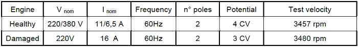
382
ICERI 2016
The Fig. 5 shows the graphic work resulting from a motor with damaged rotor
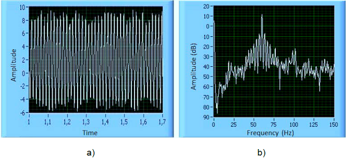
Fig.5 Current in a damaged engine: a) temporary response, b) frequency spectrum.
Fig. 5 students indicate that faults detection in motors is facilitated by increasing the engine load, since the higher the load, the lower the speed, the greater the slip, resulting in greater distance between the harmonic frequencies fundamental and those located in the sidebands, and therefore easier to distinguish failures. Therefore they recommend diagnosis of faults is performed with the engine load close to
383
ICERI 2016
the nominal.
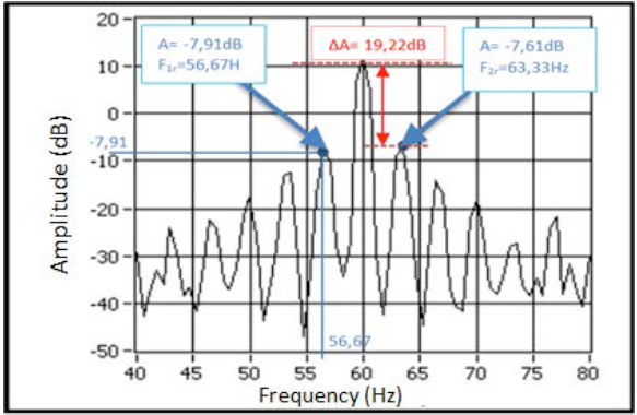
Fig.6 Test report motor damaged.
In Fig. 6, students observe current peaks at frequencies of 60Hz, and 63,33Hz 56,67Hz, corresponding to the fundamental frequency and the sidebands coincide with those expressed in the equation (13). The difference between the highest peaks of the sidebands and those of the fundamental is 19,22dB, which means that the engine has severe damage in the rotor.
384
ICERI 2016
Furthermore, students conclude that the amplitudes of the harmonic frequencies of the sidebands is
proportional to the degree of breakdown of the motor cage, therefore the difference in dB between the
magnitudes of the fundamental frequency and the harmonics will decrease as more broken bars exist
in the rotor cage [9].
Fig. 7 shows the graph obtained by the students when working with a motor with rotor without fail.
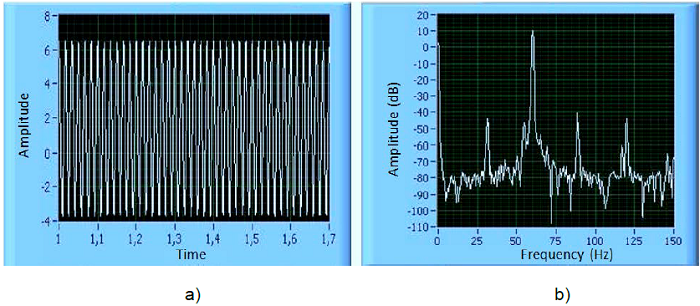
Fig.7 A healthy motor current: a) temporary response, b) frequency spectrum.
385
ICERI 2016
Fig. 8 corresponds to the report of the frequency response in the range of interest and the engine diagnosis in view of the criteria expressed in Table I, students detect that the engine is healthy.
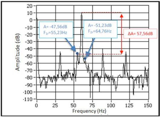
Fig.8 Test report for healthy motor
Once completed the analysis of both engines, students report that by not having the step of acquiring external data, makes it
386
ICERI 2016
possible only to evaluate the system with simulated signals or facilitated by files, limiting the amount of field tests that can be performed [10].
6 CONCLUSIONS
The methodology implemented to develop Higher Mathematics lessons with a scheme of
multidisciplinary teaching is motivating and it is closer to the why of doing of professional engineering, since knowing how to perform is a basic skill in the work life and should be encouraged during the
learning process.
By applying virtual platforms, an interconnection between computational mathematics and basic and
applied technologies develops as a means to facilitate the incorporation of knowledge and to improve
the efficiency of conventional education. It is noted that the learning process is facilitated through the
development of an appropriate language, where problematic and complex engineering situations are
proposed and solved where the investigative task is central, with a respect of learning rhythms, and
promoting collaborative learning and
387
ICERI 2016
active student participation environments.
The maintenance of computer-aided industry equipment is currently, indispensable tool in the
detection of all types of faults in induction motors. The fact that students make contact with this
experience is significant.
Today the MSCA is presented as an excellent noninvasive online monitoring alternative used to
diagnose certain problems that may occur in induction motors. This is an important tool to consider in
predictive maintenance schemes.
It is essential that the student, from initiation to completion of their chosen studies make use of
computational methods. This will strengthen the student's unified vision between mathematics and its
applications and will give them the necessary tools for their professional work.
REFERENCES
1. A. Tinnirello, E. Gago, M. Dádamo, L. Nieto, “Aspectos metodológicos para el desarrollo de capacidades básicas”, XV EMCI Nacional – VII EMCI Internacional, vol. 1, no. 1, pp. 37-46, 2009.
388
ICERI 2016
2. A. Tinnirello, E. Gago, M. Dádamo, “Designing Interdisciplinary Interactive Work: Basic
Sciences in Engineering Education”. The International Journal of Interdisciplinary Social
Sciences, vol. 5, no. 3, pp.331-334, 2010.
3. G. James, et al, “Matemáticas avanzadas para ingeniería”, Edit. Prentice HALL, México, pp.
398-426, 2002
4. R. Puche Panadero, M. Pineda Sanchez, et al ”Improved Resolution of the MCSA Method Via
Hilbert Transform, Enabling the Diagnosis of Rotor Asymmetries at Very Low Slip”, IEEE
Transactions on Energy Conversion, vol. 24, no. 1, pp. 52-59, 2009.
5. W. Thomson, M. Fenger, “Current Signature Analysis to detect induction motor faults”, IEEE
Industry Aplications Magazine, vol. 7, no. 4, pp. 26-34, 2001.
6. J. Bobadilla, P. Gomez, J. Bernal, “La Transformada de Fourier: Una visión pedagógica”.
Dialnet, vol. 1, no. 10, pp. 41-74, 2001.
7. P. O’Neil, “Matemáticas avanzadas para ingeniería”, Edit. Thomson, pp. 135-147, 2008.
389
ICERI 2016
8. V. Lajara, S. Pelegrí, “LabVIEW: Entorno grafico de programación”, Edit. Alfaomega, Madrid,
pp. 175-185, 2006.
9. D. Raheja, J. Llinas, R. Nagi, “Data fusion: Data mining based on architecture for condition
based maintenance”, International Journal of Production Research, vol. 44, no. 14, pp. 2689–
2887, 2006.
10. C. Verucchi, G. Acosta, “Técnicas de Detección y Diagnóstico de Fallos en Máquinas Eléctricas
de Inducción”, IEEE Latin American Transactions, vol. 5, no. 1, pp. 41-49, 2007.
390
EDULEARN 2017
INTEGRATING MATHEMATICS TECHNOLOGY WITH MECHANICAL
ENGINEERING CURRICULUM Descargar pdf
Alicia Tinnirello, Eduardo Gago
Universidad Tecnológica Nacional (ARGENTINA)
Abstract. The curricula of the Mechanical Engineering programs at our university include Advance Calculus at the third year of the engineering studies; the authors’ experience is that students increase their interest and their appreciation for the contents when they are involved by learning it in an applied way. With the objective to carry out these changes, we need to align the university curricula not only to the new work methods that allow intellectual development stimulation, but also to a multidisciplinary approach. This paper presents an analysis and discussion in teaching and learning environments about the integration of mathematics technology into engineering study course with the purpose to reach the competencies, knowledge
391
EDULEARN 2017
and skills required in Engineering Education. The effect of
mathematical technology on education seems to be greater in Mathematics than in other subjects.
Academic education of professional processes is challenged by necessary balance of practical
activities with academic reflection. We address this issue by discussing our experiences teaching
mathematics and the continuous improvement applied in the Mechanics Department The key objective
of this research is to identify barriers to deep mathematical understanding among engineering
undergraduates and the access to technology tools and how changed the curriculum content using
technology. Engineering faculty assume that certain concepts are taught in the mathematics courses,
but they are often not familiar with the specifics of the mathematics curriculum, or the methods utilized
(for example: terminology and context of use). Diagnostics have been performed by different
instruments applied and were identified problematics areas and specifics difficulties to integrate
technology, mathematics and engineering science. The final objective of this research is to develop a
model of curriculum integration adequate at the environment work in our University.
392
EDULEARN 2017
Keywords: Learning technology, research projects, multidisciplinary, engineering integration.
1 INTRODUCTION
New technologies are based on complex algorithms that manage to produce, through the use of
appropriate technologies, works with unexpected complexity 20 years ago. These algorithms have a
strong mathematical basis and allow conceptualize other working methods capable of solving the
problems in the practice of engineering.
The study of this new mathematic required deepen and broadening the field of knowledge. To achieve
the analysis and utilization of complex design systems and generate experimental non-linear models,
the contributions of the new math will be critical, both in the stage of formation of the engineer and his
professional life [1].
The engineer must use during the exercise of their professional activity, primarily the reasoning, in
order to understand
393
EDULEARN 2017
and solve problems with great logical components. It is therefore necessary to
focus learning on the development of processes that give the future engineer the possibility to achieve
intellectual autonomy.
Many of difficult treatment problems are multidisciplinary, including socio-economic aspects, sciences,
and engineering; they involve a large number of components, making them inherently complex.
Engineering undergraduate teaching should be appropriately structured to face these challenges.
Curricular innovations should include multidisciplinary aspects, emphasizing the points of view of
systems, and introduce engineering problems, principles, practices, and solutions from very early in
the career. There is a need to link horizontal and vertical courses by engineering problems [2].
2 THE MECHANICAL ENGINEERING PROGRAM
The structure of the existing curriculum, with subjects per year, is organized in a trunk integrator of subjects up and in a horizontal system of correlated subjects, so that students can
394
EDULEARN 2017
integrate knowledge in order of increasing complexity. An inclusive material aims to create, throughout the
career, a multidisciplinary space synthesis allowing student to understand the characteristics of the
practice of engineering, on the basis of the resolution of open problems of the Mechanical
Engineering.
The way in which the horizontal and vertical articulation of the content takes place is given, mainly,
through two areas: One 1st and 2nd level and the other 3rd, 4th and 5th level. Inclusive materials are:
Engineering Mechanics I, Engineering Mechanics II, Engineering Mechanics III, Elements of Machines
and Final Project. These subjects include the principal horizontal connection of engineering
relationships with disciplines and sciences that are issued every year and vertical from one year to
another [2].
The current curriculum is organized into four interrelated blocks: Basic Science, Basic Technologies,
Applied Technologies and Complementary Materials, being aimed at the training of professionals for
two levels of hierarchy according to the context of Argentina.
The first application includes tasks for use and operation of
395
EDULEARN 2017
consolidated technologies. The second,
development, involves tasks at the highest technical level with use of advanced technologies for which
professionals must be able to address project, design, research, development and technical
innovation. The career offers the possibility of electives subjects, in two areas, Design and
Thermomechanics in the fourth and fifth level respectively.
The basic sciences block includes the subjects of Mathematical Analysis I, Mathematical Analysis II,
Algebra and Analytic Geometry, Probability and Statistics, Physics I, Physics II, General Chemistry,
Systems of Representation, Fundamentals of Informatics and Advanced Calculus.
Subjects or binding knowledge with Advanced Calculus: Mathematical Analysis I, Algebra and Analytic
Geometry, Mathematical Analysis II, Foundations of Computer Science, Physics I and Physics II,
Thermodynamic Analysis, Mechanical Design, Solid Mechanics, Electronics and Control Systems,
Heat Technology.
396
EDULEARN 2017
3 THE EMERGENCY OF TECHNOLOGY: MATHEMATICS EDUCATION
Different works describe the various innovative experiences implemented in the classrooms of
Advanced Calculus, the career of mechanical engineering, where mediation between the content of
the subject and responses expected from the student group, was given through the gradual
incorporation, in the dictation or workshops classes, different technological applications (Mathematica,
LabVIEW, Comsol) and the use of virtual learning platforms.
Last years, have been implemented methodological strategies with different characteristics, the
activities and results achieved have being integrated as contributions made to the training in
engineering.
Educational interventions were developed by using technological applications available to explore
concepts of modeling, estimation of parameters, numerical simulation and case analysis, pursuing
better understanding of concepts and procedures.
Besides, the results achieved by the students were emphasis
397
EDULEARN 2017
after using technological applications to validate, verify properties, classify or perform complicated calculations in different subjects, (complex variable function, Laplace transform, Series and Fourier Transform) [3].
4 CHANGES AT THE CURRICULUM CONTENT
The University curriculum reform was based, among the following issues: The need to strengthen and
enhance the graduate profile, in accordance with the requirements of knowledge and skills demanded
by the society; and in addition, to guide the methodological approach of the programs toward a new
kind of teaching [4].
In this context, the Engineering Federal Council projects a curricula reform. The most relevant
changes of the proposal are: Train engineers with a general formation, balanced between scientific,
technological, management and humanist aspects. Following these changes, the Superior Council of
the Technological University approved by resolution of the Board of Governors a New Curriculum
Design.
Among the significant changes in the New Curriculum Design
398
EDULEARN 2017
are the reduction of the curricula of engineering careers that go from 6 to 5 years of nominal duration; the commitment with the need to achieve a strong student training in basic cycle of engineering careers; to homogenize the knowledge; to make changes in the subjects content in basic cycle; and to introduce the computational tools in teaching, to the realization of practical work of all subjects in the area of Mathematics [5]. Use of technology made it possible to make more explicit the role of modes of representation. In particular, the way in which the complementarity between graphic, numerical and symbolic representation, produce best comprehension using technology and help develop coordination processes. Thus, the descriptions of the construction process followed by students have allowed relating aspects of the particularization to the reflective abstraction derived from the modes of representation in construction knowledge. These early educational experiences continued with intervention and interaction activities with students, inside and outside the laboratory, through virtual platforms, always favoring the approach and requests. The use of ICTs in general, relied on the publication of information in sites accessible over the Internet, so that students
399
EDULEARN 2017
are acquiring skills of search and self-information and different forms of access; the distribution of some materials for study and report generalized; a communication space was developed on an educational platform and these means, management, planning and monitoring the course, enabling information in exchange forums.
5 IDENTIFYNG DIFFICULTIES AND BARRIERS
Learning tasks should approximate in some way to the approach of the complexity requirements,
leading to subversion when required, the simplicity in the thinking of the student and its application into
practice; not a simple debate or practical exercise, it is studying the teaching process by specifying the
mechanisms and mindsets established in order to locate where do make a change [5].
Sciences of complexity explore spaces, open horizons and anticipate processes, phenomena and
dynamics, it is in this sense that the use of modeling and simulation reveals essential to explore
models, solutions space, with crosses among them, for the study of behaviors characterized by
instability,
400
EDULEARN 2017
uncertainty, adaptation, non-linearity.
To analyze the profile of the entrants to the career and to take into account the performance in the
University seminar, we arrived at the conclusion that the students were admitted to the University with
low levels in certain competitions such as ability to abstraction and analytical thinking, among others.
A diagnostic study was developed to measure levels of mathematical knowledge gained in previous
years perceived by Advanced Calculus Engineering students. The Mathematical knowledge search
consisted of five dimensions: Integration, Differentiation, General subject, Graphics and Limit, related
to subject of Mathematics curriculum [4], [5], [6].
There was a very significant difference between the students that successfully have completed the
Mathematical Analysis I, Mathematical Analysis II courses during the 1st two years of the careers and
those failing those courses. To solve the difficulties to understand concepts view in previous years,
practical sessions were implemented at the beginning of Advance Calculus where several applications
were showed through special material referred to modeling physical systems and to explain the
significant of different mathematical tools in
401
EDULEARN 2017
engineering.
6 INTERACTIVE/VIRTUAL LEARNING ENVIRONMENTS
What would an ideal class, adjusted to these changes? When the class is developed in an
atmosphere of construction knowledge, the virtual lab plays a key role in this new model of teaching
and learning. The introduction of software in problem solving processes influences on the sequencing
of the steps which are considered and the criteria which are built for such resolution.
Computer-based education allows us to develop skills in students promoting critical thinking,
facilitating the interpretation and limitations of the theory, i.e. experimental study thus prepares
students for professional challenges where these tools play an essential role in the Industry.
The designed activities were focused to incorporate various strategies such as: Simulated signals
generated in physical systems due to functions of one or more variables representing characteristics or behavior of any physical process, systems modeling as devices that are responsible for
transforming
402
EDULEARN 2017
the signals responses producing others or any desired result, as well as build and
develop skills in management methodologies and mathematical tools for signals treatment in
continuous and discrete time systems, in the temporary or frequency field, deterministic or stochastic.
Identified strategies are designed to develop skills in students to adopt a style of active learning that
favors the ability to deal with risks and a competent behavior to deal with difficult situations, for
example, requiring discover solutions, manage conflicts, give feedback and learn to delegate.
Modeling and simulation are, require or imply mathematical formalization (previous) work, but this is
not always true, sometimes the mathematization can be done later as a verification or demonstration
of what has been modeled or simulated. It is necessary to consider that simulation and modelling
demand prior work, conceptual or theoretical, that leads to analyze algorithmic or computational
problems.
7 ADVANCE CALCULUS AND APPLICATIONS
Examples of assignment work and computer projects
403
EDULEARN 2017
7.1 Modeling and simulation of mathematical tools used for faults in bearings
We analyzed the different existing methods oriented to the study of failures in mechanical systems
through spectral and temporal models: Waveform Graphics and spectra using the FFT analysis.
The methodology used was: Create signals by means of simulated data, presentation of the wave
patterns and the corresponding spectrum, addition of stochastic noise from generators, spectral
analysis of signals with noise and presentation of parametric models [7].
It was investigated on the different types of spectral frequency characteristic of failures such as:
imbalance, misalignment, looseness, friction between moving parts, failure of bearings, problems in
the engagement of a couple teeth, rotors of electric motors with broken or defective bars, etc. also was
interpreted the influence of the phenomenon of resonance in the spectrum of frequencies.
We provide an activity to the students to deal with real problems through simulation and perform a
statistical analysis of data by using the technological tools to integrate the
404
EDULEARN 2017
knowledge of the calculation
of probabilities and dynamic models and apply it to real processes.
Dynamically signals were simulated for the study of vibrations in rotating equipment, to display
different analysis techniques and mathematical models involved. Patterns of different signs were
analyzed to incorporate prior knowledge about the behavior of the mechanical systems operating in
theoretical conditions of functioning. Simulated signals were compared with the real signals, checking
the signals with the patterns when noise is added that disturb the output vibration signal.
They simulate signals with and without noise, the noise was incorporated by stochastic generators.
This procedure provides a more realistic estimate signal which can deal with the ones that show the
measuring equipment, allowing a more genuine comparison of the graphics information that they
provide.
The results of these works are shown below:
a) Patterns of behavior of a signal of a gear with wear, sine wave and equation mixture of
harmonics without and with noise, Fig. 1, Fig. 2.
405
EDULEARN 2017
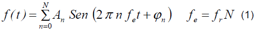
being
 phase angle and N number of gear teeth [3], [8].
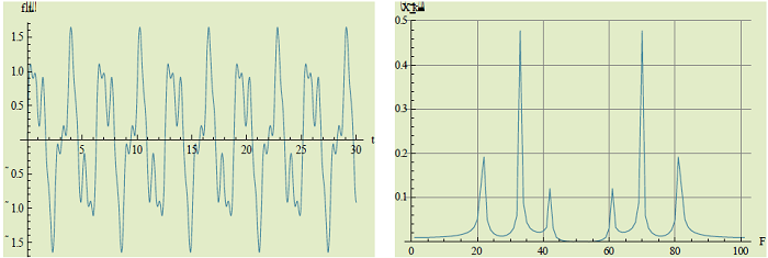
 Figure 1. Gear SignalFigure 2. Spectral Analysis
406
EDULEARN 2017
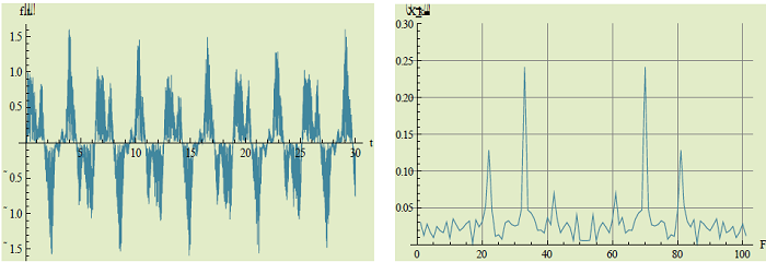
Figure 3. Gear signal with Figure 4. Spectral analysis
noise
Figure 4. Spectral analysis
noise  with noise
b) Axis of rotation slide: Equation of sine wave with changes in frequency amplitude
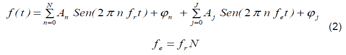
being
, phase angle and Aj the j-th harmonic amplitude [3].
407
EDULEARN 2017
Figure 5. Misaligned axis. Signal and spectral analysis without noise
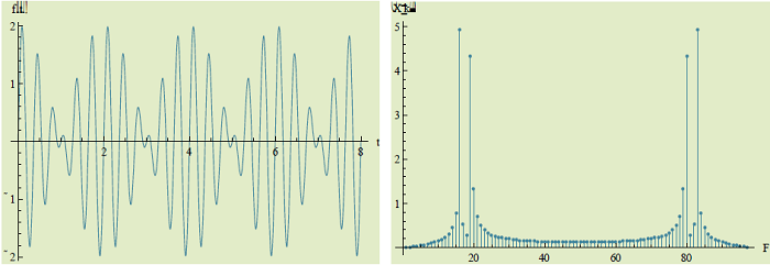
Figure 6. Misaligned axis. Signal and spectral analysis with noise
408
EDULEARN 2017
7.2 Failures that occur in an induction motor: Simulation of an electrical signal
The objective is the signal analysis rather than the techniques of data acquisition and LabVIEW is used as a platform for simulation. Through the front panel students watch the simulation perform by the analysis of the simulated signal coming from the engine, illustrated in Fig.7:
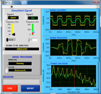
Figure 7. Front panel
Since the student interest is focused on signal analysis, rather
409
EDULEARN 2017
than technical data acquisition, and considering that LabVIEW was choosing as a deployment platform intentionally, it facilitates the acquisition, signal conditioning and testing the signals stored [9].
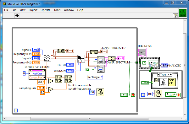
Figure 8. Blocks diagram
Fig. 9 was analyzed to detect faults in motors provided with increasing engine load, since the higher load produce lower
410
EDULEARN 2017
speed, greater the slip, resulting in more distance between the fundamental harmonic frequencies and those located in the sidebands, and therefore easier to distinguish failures. Therefore was concluded that diagnosis of faults is performed with the engine load close to the nominal [10], [11].
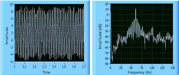
Figure 9. Damaged engine: temporary response and frequency spectrum.
In Fig. 10, students observe current peaks at frequencies of 60Hz, and 63,33Hz 56,67Hz, corresponding to the fundamental frequency and the sidebands matches with those expressed in
411
EDULEARN 2017
previously works. The difference between the highest peaks of the sidebands and the fundamental is 19,22dB, which means that the engine has severe damage in the rotor [12], [13].
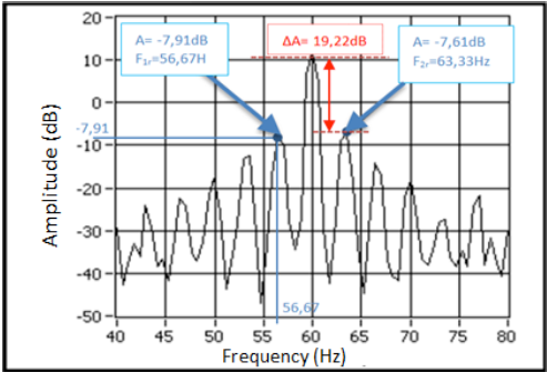
Figure 10. Test report of a motor damaged
7.3 Design of an air heater, simulation and modeling with COMSOL
Multiphysics
The problem presented here is the design of heat transmission
412
EDULEARN 2017
equipment development in a laboratory
class as an example task for mechanical engineering.
It was very interesting the treatment in the class of this engineering application as the air heaters are
an interesting option to increase the performance of the cycle responsible for generating steam.
The project consists in the air heater design, where the fluid enters from the top and comes in contact
in descending order with the gas pipes of heat transmission, which are placed in the form of a
labyrinth, the design allows the contact of the air with pipes across its surface, while the air outlet is
located at the bottom.
Students work with the Comsol Multiphysics simulation platform that represents through their
interactions what happens with the fluid when it's exposed to different conditions of work.
Specifically, technology used is CFD (Computational Fluid Dynamics) of COMSOL. This module is designed for the solution and simulation of fluid flow problems ranging from a single stage laminar flow to a turbulent flow and the resolution of problems of heat transfer, either by conduction, convection or
radiation [14].
This module includes numerical methods and
413
EDULEARN 2017
algorithms to replace the systems of partial differential equations in algebraic systems equations to solve using a computer [10]. The work carried out can be seen in Fig.11 (a), where it is displayed how the temperature varies while the air enter in contact with the tubes, while in Fig.11 (b) indicated by a temperature graph characteristic points in the design equipment. In Fig. 12 is observed another simulation to increase the temperature to 60°C studying air temperature of the outgoing air.
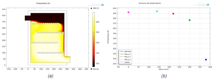
Figura 11. Temperature variation T0 = 25 °C
414
EDULEARN 2017
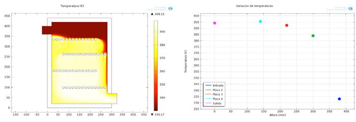
Figura 12. Temperature variation T0 = 60°C
It was also discussed, the variation of the speed of the fluid, Fig. 13, and the increase with the increase of temperature. The simulation design allows perform a real analysis of the pressures, variation of density, internal energy, etc. These are other features that can lead to an optimization of fluid flow analysis [15], [16].
415
EDULEARN 2017
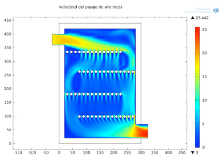
Figura 13. Velocity variations. V0 = 17,5 m/s
Using Comsol showed the importance of technologies implementation to study the main phenomena that occur in the nature of fluids flow and the heat transmission, in a particular context. The simulation results it can clarify in what way it behaves a fluid exposed to different conditions and analyze the full behavior of the same in its path. It follows that the use of the virtual platform streamlines the study of physical phenomena, contrasting the methods used to verify the experimental results.
416
EDULEARN 2017
8 CONCLUSIONS
The teaching activity based on these types of integration discipline allows the concepts, theoretical frameworks, procedures and other elements with which they have to work with teachers and students are organized around units more global, conceptual and methodological structures shared by several disciplines. The academic activities of integration discipline contribute to the consolidation of certain values in teachers and students: flexibility, trust, patience, intuition, divergent thinking, sensitivity toward other people, acceptance of risks, learns to move around in the diversity, accept, new roles, among others. The work in Advance Calculus with technology has created a new relationship between the teachers of basic and applied technologies and research groups, which promotes the interaction, aimed at achieving the multidisciplinarity in the process of teaching, the application of new technologies, the transfer to the classroom of research for the best treatment of various subjects; and work in conjunction with the purpose of improving the quality of teaching, and thus to achieve the curriculum objectives. Besides this form of work
417
EDULEARN 2017
is closer to the way students will face in their professional life.
ACKNOWLEDGEMENTS
The authors would like to express their recognition to the students Lucas D’Alessandro and Mariano Valentini for their performance during the development of their project work.
REFERENCES
1. A. Tinnirello, E. Gago, L. D’Alessandro, M. Dádamo, “Virtual Instruments Integrating
Mathematical Modeling for Engineering Education”, Proceedings of 9th annual International
Conference of Education, Research and Innovation, pp. 255-264, 2016.
2. R. Posada Álvarez, “Formación Superior Basada en Competencias, Interdisciplinariedad y
Trabajo Autónomo del Estudiante”, Revista Iberoamericana de Educación, 2011.
3. G. James, et al, “Matemáticas avanzadas para ingeniería”, México, Edit. Prentice HALL, pp.
178-202, 2002.
418
EDULEARN 2017
4. V. Macchiarola, “Currículum basado en competencias. sentidos y críticas”, Revista Argentina de
Enseñanza de la Ingeniería, Vol. 8,Issue 14, pp. 39-46,2007.
5. G. Bischof, E. Bratschitsch, A. Casey, Domago Rubesa. (2007). “Facilitating Engineering
Mathematics Education by Multidisciplinary Projects”, Journal of American Society for
Engineering Education. 2008
6. B. Prepelita-Raileanu, “Social Software Technologies and Solutions for Higher Education”,
Proceedings of the 8th WSEAS International Conference on Education and educational
Technology, 2009.
7. A. Tinnirello, “Stochastic Models in Engineering Quality Problems”, Journal WSEAS
TRANSACTIONS on SIGNAL PROCESSING, Issue 2, Vol. 2, 2006.
8. A. Tinnirello, S. De Federico, “Modelos Espectrales para el Análisis de Fallas en Sistemas
Mecánicos”, Congreso Argentino de Ingeniería Mecánica, 2008.
9. V. Lajara, S. Pelegrí, “LabVIEW: Entorno grafico de programación”, Madrid, Edit. Alfaomega,
pp. 175-185, 2006.
419
EDULEARN 2017
10. K. Astrom, R. Murray, “Feedback Systems: An Introduction for Scientists and Engineers”,
U.S.A., Princeton University Press, pp. 201-226, 2009.
11. R. Randall, “State of Art in Monitoring Rotating Machinery”, Journal Sound and Vibration, pp 10-
16, 2004.
12. A. Fernández, J.Bilbao, I. Bediaga, A. Gastón, J. Hernández, “Feasibility study on diagnostic
methods for detection of bearing faults at an early stage”, WSEAS International conference on
Dynamical Systems and Control, pp. 113-118, 2005.
13. Tinnirello. A., Gago, E., D’Alessandro, L., Szekieta, P., “Diagnosis of Rotor Failures Current
Power Induction Motors by Spectral Analysis Methods”, International Journal of Circuits and
Electronics, pp. 191-198, 2016.
14. A. Batatunde, A. Ogunnaike, W. Harmon Ray, “Process Dynamics, Modeling, and Control”
Oxford University Press, pp. 430-459, 1994.
15. B. Orgunnaike, W. Harmon Ray, “Process Dynamics, Modeling, and Control”, Oxford, EE. UU,
Oxford University Press, pp. 430-459, 1994.
420
EDULEARN 2017
16. K. Ogata, “Ingeniería de control moderna”, Madrid, Edit. Pearson, pp. 178-202, 2010.
17. R. TORRES, J. GRAU. “Introducción a la mecánica de fluidos y transferencia de calor con
COMSOL Multiphysics”, España, Edit. Addlink Software Científico S.L., 2007.
18. Y. Lin, “Grey Systems. Theory and Application”. Edit. Springer-Verlag, Berlin, pp. 475-479,
2011.
19. Thanagasundram, S. and Soares Schlindwein, F., “Autoregressive Order Selection for Rotating
Machinery”, International Journal of Acoustics and Vibration, Vol. 11, N° 3, 2006.
20. W. Wang, “Autoregressive model-based diagnostics for gears and bearings”, British Non-
Destructived Testing and Condition Monitoring, Vol. 50, Issue 8, pp. 414-418, 2008.
21. Y. Zhan, V. Makis, A. Jardine, “Adaptive model for vibration monitoring of rotating machinery
subject to random deterioration”, Journal of Quality in Maintenance Engineering, Vol. 9, Issue 4,
pp. 351-375, 2003.
421
IJELS 2017
INTRODUCING DISCRETE DYNAMIC SYSTEMS IN ALGEBRA TEACHING PROCESS Descargar pdf
Paola Szekieta, Alicia Tinnirello, Eduardo Gago
Computer and Basic Sciences Laboratory
Universidad Tecnológica Nacional – Facultad Regional Rosario
Zeballos 1341, Rosario, Santa Fe
ARGENTINA
paolasz@gmail.com, amtinni@gmail.com, eagago@gmail.com
Abstract. The aim of this work is to present a university classroom experience where the concepts of discrete dynamic systems are introduced in Algebra and Analytical Geometry subject with the purpose of using simulations where matrices are involved, in this case cellular automaton models are used as a dynamical system with discrete values in space, time and state. In this experience, computer scientists and mathematicians work together to carry out interdisciplinary projects which present discrete data management to first-year engineering students. Taking into account the fact that cellular automata have been used in
423
IJELS 2017
different disciplines successfully, the authors of this paper consider introducing its concepts and applications in engineering teaching process.
Keywords: Discrete dynamic systems, cellular automata, computational mathematics
1 INTRODUCTION
This innovative activity is carried out by the Computer Laboratory of Basic Science of our University in order to introduce the mathematical developments to discrete variable events. The starting point is not whether content or processes have priority in the learning process, but making sure that learning becomes meaningful and functional. Computer tools currently available are used to develop students’ skills in the design of mathematical modeling with one discrete variable by teaching the fundamental basics of cellular automata (CA) in
424
IJELS 2017
order to show the existing relations with symbolic calculus and the applications which these have with system resolution and modeling.
These applications are wide, ranging from microscopic simulations of Physics and Biology to macroscopic simulations of social and geological processes (Our translation) [1].
CAs are among the simplest mathematical representations of dynamical system that consist of more than a few – typically nonlinearly – interacting parts [2].
As such CAs are extremely useful idealizations of the dynamical behavior of many real systems, including physical fluids, molecular dynamical systems, natural ecologies, military command and control networks , economy fire spreading, epidemiology and many others [3] [4]. Because of their underlying simplicity CAs are also powerful conceptual engines with which to study general pattern formation [2].
CAs consists of a regular array of identically programmed units called cells or sites that interact with their neighbors’ subjects to a finite set of rules prescribed by local transitions. All sites make a regular lattice and they evolve in discrete time steps as each site assumes a new value based on the values of some local
425
IJELS 2017
neighborhood of sites and a finite number of previous time steps [5].
As M. Resnick suggests, the performance of this model is governed, not by a centralized authority but by the local interaction among decentralized components [6].
2 CONCEPTS OF CELLULAR AUTOMATA
According to Wolfram: CA are examples of mathematical systems constructed from many identical components, each simple, but together capable of complex behavior [7]. Some basic characteristics as regards the structure which the CA has are described. They represent a discrete system where the space, the time and the states of the system are all discrete and have the following properties: Space is represented by a regular lattice in one, two, or three dimensions; each site, or cell in the array of the CA can be in one of a finite number of states [8].
2.1 Neighborhood
The neighborhood of a lattice site consists of the site itself and
426
IJELS 2017
its nearest neighbor sites, called neighbors. Two kinds of neighborhoods are commonly defined for a rectangular lattice: A Von Neumann neighborhood consists of the site and the four nearest neighbors, situated above, below, right and left as shown in Fig.1 below.

Fig.1 Von Neumann neighborhood
A Moore neighborhood consists of the site and the eight nearest neighbors as shown in Fig.2 below.
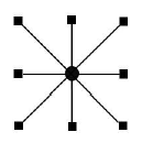
Fig.2 Moore neighborhood
427
IJELS 2017
2.2 Lattice Boundaries. Periodic Boundaries
The nearest neighbors of sites along the sites of a lattice are determined differently for various boundary conditions. The way these conditions are defined will impact directly on the automata behavior. The periodic boundaries which are used in the modeling of the CA used in the target activity are defined. To illustrate this criterion, the corresponding Moore neighborhoods are shown below for each site in the following simple lattice:

This type of boundaries is defined when the neighbors of the sites on the borders of the lattice are set in the following way:

428
IJELS 2017

The nearest neighbor left of a site on the left border is the site in the same row on the right border. In the same way, the neighbors on the right of the cells on the right border are analyzed. The nearest neighbor above site on the top border is the site in the same column on the bottom border. In the same way, the neighbors on the bottom order are analyzed.
2.3 Evolution Rule
Another basic component worth mentioning is the Evolution Rule which defines the state of each cell according to the immediate previous state of the neighborhood. This evolution is determined by a mathematical function which captures the
429
IJELS 2017
influence of the neighborhood over the target cell.
2.4 Virtual Clock
The virtual clock is a clock which will generate simultaneous ticks to every cell indicating that the evolution rule must be applied to modify or maintain the state of the cell. This component fulfills the parallelism condition, i.e. all the cell area updated at the same time [9].
3 GAME OF LIFE ALGORITHM
The Game of Life, which was created by the British
mathematician J. H. Conway in 1970s, is the most
famous CA. More computer time has been spent on
running this game than on any other calculation and
it was the first program executed by the Connection
Machine, the world's first parallel computer.
According to Gaylord & Wellin: it is the forerunner
of so-called artificial life (or a-life) systems which
are of great interest today, not only for their
biological implications, but for the development of
so-called intelligent agents for computers [5].
430
IJELS 2017
This automaton is a game of cero players, which
implies that its evolution is determined by its initial
set-up and there is no need of any further data entry.
The game unfolds over a bidimensional grid as the
game board. Each position on the board is called
cell and it has 8 neighbor cells which are the nearest
to each of them, including the diagonal ones (Moore
neighborhood). The cells have two states, living or
dead, which are represented by the numbers 1 and 0 respectively. The number and arrangement of living
cells on the board evolve along the discrete time
units. All cell states are taken into account to
calculate their state in the following time. All cells
are updated simultaneously. The transitions depend
on the number of neighbor cell which are alive. A
dead cell with exactly 3 living neighbors will be
born in the next turn. If a living cell has 2 or 3
neighbor living cells, the following turn it will still
be living. In any other case, it will die or remain
dead due to loneliness or overpopulation.
The game set out will continue until 2 identical
consecutive states are obtained, or rather, until a
certain number of predetermined transitions are
reached.
To start the modeling of this game, an initial cell
array over the
431
IJELS 2017
board is set at the time t = 0, represented by the following grid:
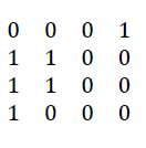
Fig.3 below shows each element on the board and its neighbors considering a Moore neighborhood with periodic boundaries.
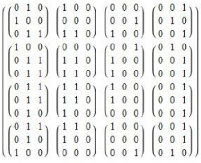
Fig.3 Moore neighborhood on initial grid
432
IJELS 2017
It is possible to determine the number of living neighbors in each of the initial positions, counting the numbers of living neighbors which are around each cell:

Comparing the state of each cell of the game
board in time t and the number of living neighbors,
the following state in time t+1 can be set up.
Fig.4 below shows the transition from initial time
t= 0 to t = 1. To visualize some examples, if we
consider de state of de second element on first board
row, it has 3 living neighbors so this cell will be
born at t = 1 but first cell on third row of the board
will be dead at next turn due to overpopulation.
433
IJELS 2017
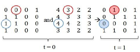
Fig.4 Evolution from t = 0 to t = 1
Fig.5 shows evolution from t = 1 to t = 2. On the last row of the game board two cases of surviving rules are highlighted.
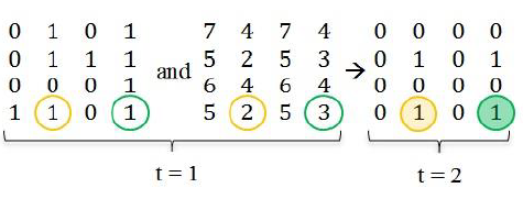
Fig.5 Evolution from t = 1 to t = 2
At the time instance t = 3, a board with all dead cells is obtained as shown in Fig.6 below. The following turn, time t = 4, the same result will be obtained, so the game will finish by obtaining two consecutive similar states.
434
IJELS 2017
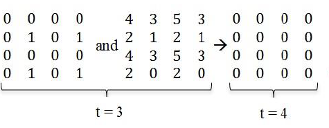
Fig.6 Evolution from t = 3 to t = 4
4 LABORATORY PROJECT: DEFINING AND DEVELOPING A COMPUTATIONAL SIMULATION MODEL
In the context of meaningful learning, the students'
activities must be oriented in a school system based
on research and development of appropriate
strategies for connecting and integrating the computational mathematics and the basic
technologies and applied in Engineering to promote
the multidisciplinary approach to the curriculum
content corresponding to the plans of study, aiming
to train professionals capable of solving complex
models with the use of technologies.
The existence of simulation tools transformed the
programming
435
IJELS 2017
environments toward more
collaborative spaces, with the updated listings of
increasingly complex systems but with broad
application in the various areas that comprise the
engineering, it is possible to design methodological
strategies that integrate the knowledge of the
compartmentalized disciplines.
The developments that have experienced the
mathematical software and the affinity that the
students have to be linked with the technologies,
imposes on the university teachers makes the effort
to transform the teaching-learning process in the
process of learning investigating [10].
The present experience shows the representation
of the Game of Life using specific software
(MATHEMATICA, Wolfram Research). To do this,
the board and the way neighborhood for each cell is
obtained as well as the transition rules should be set
up.
The board is represented by a square matrix of
order 4 St, and each of its entries is the state of a
particular cell at a given time 𝑡.
The following step is to define the function
which returns the number of neighbors alive of each
cell of the board. To model this automaton, the
Moore neighborhood is considered which
436
IJELS 2017
is made up by the 8 neighbors around the position which is often identified with a cardinal point according to the position of the central cell: north, northeast, east, southeast, south, southwest, west and northwest. Fig.7 below shows this Moore neighborhood.
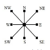
Fig.7 Moore neighborhood
It is possible to obtain a matrix that shows a particular neighbor by performing elementary operations on St. For example, to obtain a matrix Nt whose elements nij represent north neighbor of each site sij in St at a certain time 𝑡, it is necessary to move down every row on St by properly interchanging them. Ec. (1) shows N0 that is north neighbors of< each site sij at time 𝑡 = 0.
437
IJELS 2017
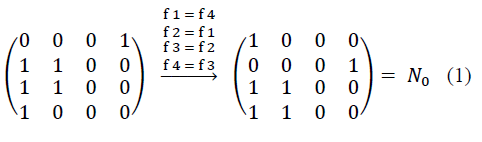
To find the matrix NE0 whose elements represent the neighbor in the Northeast position of each sij in S0, first move the rows (f) downwards as shown in (1) above and then, on this resulting matrix, interchange columns (c) to the left. See (2) below.
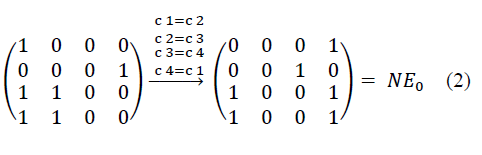
Similarly, it is possible to obtain matrices that show a particular neighbor for each position in the state space and therefore to know the number of living neighbors of sij adding these 8 matrices of neighbor positions.
438
IJELS 2017
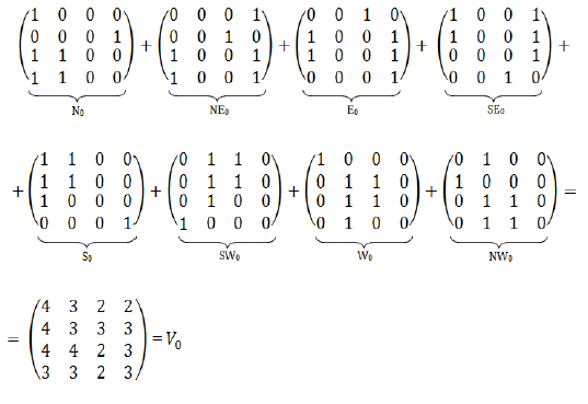
Fig.8 Number of living neighbors’ matrix at 𝑡 = 0
Fig.8 above shows how to obtain number of
living neighbors matrix at time 𝑡 = 0.
Analyzing values of homologous elements on St
and Vt, the next state into which sij will evolve can
be obtained.
The evolution rule is function to the state of a
cell sij and the number of living neighbor which it
has.
439
IJELS 2017
Rule
[stij : cell state sij , vtij : number of
living neighbors sij] = st + lij .
A living site with two living nearest neighbor
sites remains alive: Rule [1,2] = 1.
Any site (no matter if living or dead) with three
living nearest neighbor sites stays alive or is born:
Rule [_,3] = 1.
All other cases, one cell either remains dead or
die: Rule [_, _] = 0.
The following matrices: S0 ; S1 ; S2 ; S3 ; S4 show
the consecutive states which the game reaches at
each instance 𝑡. Matrices can be represented
graphically with a black site for living cells and a
white one for dead cells. Fig.9 shows both
representations.
440
IJELS 2017
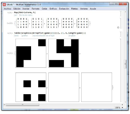
Fig.9 Game consecutive states
These rules are simple enough for anyone to understand, yet the Game of Life leads to an endless number of different patterns, and to significant complexity [11]. It is interesting to observe different these patterns or life forms. Students investigated these patterns and modified initial set-up to watch diverse evolution processes of the game. Laboratory work classes are an integral part of any educational program and
441
IJELS 2017
their purpose is
bringing the students closer to real situations of the
area of studies.
Some of these cases are shown below Fig.10,
Fig.11 and Fig.12.
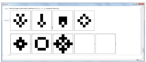
Fig.10 Cross pattern
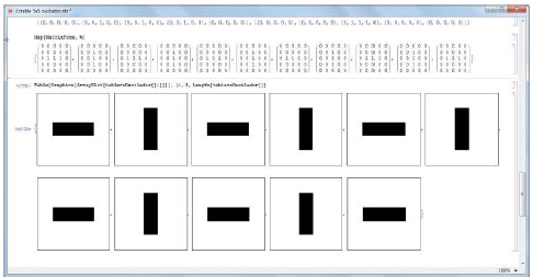
Fig.11 Oscillator
442
IJELS 2017
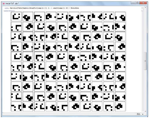
Fig.12 Spaceship pattern
5 Engineering application: Pollutant
diffusion in a liquid form
CA application is the pollutant diffusion in a liquid form, for example the water flows which are presented in the projects of environmental remedial. In fact, this tool can be useful to guide
443
IJELS 2017
and support the processes applied to purify contaminated water. It is not easy to obtain a numeric solution from a mathematical expression for such a phenomenon. However, there are ways to approach the problem by mathematical modeling of fluid transport: some of these methods will be studied in higher courses of engineering careers, CAs often provide a simpler tool that preserves the essence of the process by which complex natural patterns emerge [12].
Fig.13 Initial concentrations of pollutant
Fig.13 shows a model of a liquid form with high pollutant concentrations on the high left corner of the analyzed section.
444
IJELS 2017
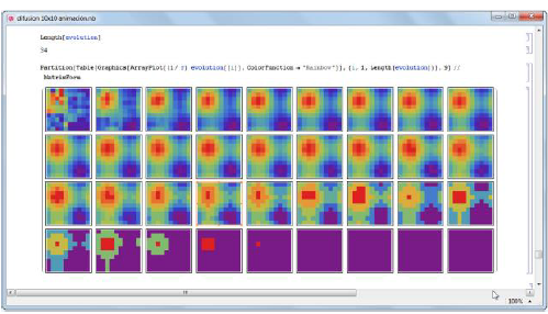
Fig.14 CA Simulated Pollutant Diffusion
Fig.14 above shows the evolution of the pollutant
diffusion throughout time until all section under
analysis is covered and a constant concentration is
reached:
Students are required to interpret the software
graphic output of pollutant diffusion and to compare
it with other software outputs which can result from
changing the initial configurations of the pollutant
concentrations. This mathematical model is applied
to understand the distribution of pollutants by
formulating a 2D diffusion.
445
IJELS 2017
4 CONCLUSION
The CAs have been used in different disciplines
successfully. Currently, attention is raised towards
the development of models which can carry out
complex tasks such as cryptography, image
processing and turbulence analysis, among others.
This is the reason why we consider important to
introduce CA concepts and applications in
engineering teaching, taking as a starting point the
study of mathematical models with discrete variable
systems.
By introducing experiences as the ones described
in the present paper for Algebra and Analytical
Geometry, we search for a change of perspective
which can see algorithms as a mathematical key
activity and computer science as complementary
knowledge to run those algorithms and manage their
outputs.
Strategy design is highlighted as the outset of the
study of mathematical models to solve discrete
variable problems integrating the computational
mathematics with the technological areas of the
engineering curriculum while incorporating new
learning styles.
446
IJELS 2017
REFERENCES
1 G. Merino, Use of a Cellular Automaton to
Create a Diffusion Model of Pollutants in a
Soil-Water System. Journal of Mathematics:
Theory and Applications, Vol.18, Nro.1, 2011,
pp. 63-76.
2. A. Ilachinski, Cellular Automata: A Discrete
Universe, World Scientific, 2001, pp. 175-185.
3. J. Quartieri, N. Mastorakis, G. Iannone, C.
Guarnacci, A Cellular Automata Model for Fire
Spreading Prediction, Proceedings of 3rd
WSEAS International Conference on Urban
Planning and Transportation, 2010, pp. 173-
179.
4. M. Dascalu, G. Stefan, A. Zafiu, A. Plavitu,
Applications of Multilevel Cellular Automata in
Epidemiology, Proceedings of the 13th
WSEAS international conference on Automatic
control, modelling & simulation, 2011, pp.
439-444.
5. R. Gaylor, P. Wellin, Computer Simulations
with Mathematica: explorations in complex
physical and biological systems. Springer-
Verlag, 1995.
447
IJELS 2017
6. M. Resnick, Turtles, Termites, and Traffic
Jams, MIT Press, 1994.
7. S. Wolfram, Cellular automata as Model of
Complexity. Nature, Vol.311, 1984, pp. 419-
424.
8. R. Gaylor, K. Nishidate, Modeling Nature:
Cellular Automata Simulations with
Mathematica, Springer-Verlag, 1996.
9. J. Muñoz, Autómatas Celulares y Física
Digital, Memorias del Primer Congreso
Colombiano de Neuro Computación. Academia
Colombiana de Ciencias Exactas, Físicas y
Naturales, Bogotá, 1996.
11. T. Ostoma, M. Trushyk, Cellular Automata:
Theory and Physics. A New Paradigm for the
Unification of Physics, Cornell University
Library, 1999.
12. S. Wolfram, Computer Software in Science and
Mathematics,
448
IJMMMAS 2017
COMPUTATIONAL MATHEMATICS IN ALGEBRA TEACHING PROCESS Descargar pdf
Paola A. Szekieta, Alicia M. Tinnirello, and Eduardo A. Gago
Abstract. In this work the authors present a mathematic laboratory experience where the concepts of discrete dynamic systems are introduced in Algebra and Analytical Geometry subject with the purpose of using computer packages to familiarize students with recent developments at an early stage, in this case cellular automaton models are used as a dynamical system with discrete values in space, time and state. In this experience, computer scientists and mathematicians work together to carry out interdisciplinary projects which present discrete data management to first-year engineering students. Starting from the theoretical concepts, different cellular automata have being presented with interesting applications for connecting and integrating the computational mathematics in engineering teaching process.
451
IJMMMAS 2017
Keywords: Discrete dynamic systems, cellular automata, computational mathematics.
1 INTRODUCTION
Simple problems can be formulated, increasing the difficulties using simple programming assignments algorithms and generating a gradually process where students arrive at complex works that would have involved time-consuming efforts without computer support.
This innovative activity is carried out by the Computer Laboratory of Basic Science of our University in order to introduce the mathematical developments to discrete variable events. The starting point is not whether content or processes have priority in the learning process, but making sure that learning becomes meaningful and functional.
Computer tools currently available are used to develop students’ skills in the design of mathematical modeling with
452
IJMMMAS 2017
one discrete variable by teaching the fundamental basics of cellular automata (CA) in order to show the existing relations with symbolic calculus and the applications which these have with system resolution and modeling.
These applications are wide, ranging from microscopic simulations of Physics and Biology to macroscopic simulations of social and geological processes (Our translation) [1].
CAs are among the simplest mathematical representations of dynamical system that consist of more than a few – typically nonlinearly – interacting parts [2].
As such CAs are extremely useful idealizations of the dynamical behavior of many real systems, including physical fluids, molecular dynamical systems, natural ecologies, military command and control networks , economy fire spreading, epidemiology and many others [3] [4]. Because of their underlying simplicity CAs are also powerful conceptual engines with which to study general pattern formation [2].
CAs consists of a regular array of identically programmed units called cells or sites that interact with their neighbors’ subjects to a finite set of rules prescribed by local transitions. All sites make a regular lattice and they evolve in discrete time steps as each
453
IJMMMAS 2017
site assumes a new value based on the values of some local neighborhood of sites and a finite number of previous time steps [5].
As M. Resnick suggests, the performance of this model is governed, not by a centralized authority but by the local interaction among decentralized components [6].
Researchers have tried to develop different algorithm which can model different applications, in the beginning of the eighties Stephen Wolfram studied a family of simple one-dimensional CA rules, famous as Wolfram rules, and these simplest rules are capable to represent complex systems.
According to Wolfram: CAs are examples of mathematical systems constructed from many identical components, each simple, but together capable of complex behavior [7]. Some basic characteristics as regards the structure which the CA has are described. They represent a discrete system where the space, the time and the states of the system are all discrete and have the following properties: Space is represented by a regular lattice in one, two, or three dimensions; each site, or cell in the array of the CA can be in one of a finite number of states [8].
454
IJMMMAS 2017
2 BACKGROUND ON CELLULAR AUTOMATA
From a theoretical point of view, some main concepts play an important role in CAs models:
A. The physical environment
This defines the universe on which the CA is computed. This underlying structure consists of a discrete lattice of cells with a rectangular, hexagonal, or other topology. Typically, these cells are all equal in size; the lattice itself can be finite or infinite in size, and its dimensionality can be 1 (a linear string of cells called an elementary cellular automaton), 2 (a grid), or even higher dimensional. In most cases, a common—but often neglected—assumption, is that the CAs lattice is embedded in a Euclidean space [3].
B. The cells’ states
Each cell can be in a certain state, where typically an integer represents the number of distinct states a cell can be in, e.g., a binary state. Note that a cell’s state is not restricted to such an
455
IJMMMAS 2017
integer domain; a continuous range of values is also possible, in which case we are dealing with coupled map lattices. We call the states of all cells collectively a CAs global configuration. This convention asserts that states are local and refer to cells, while a configuration is global and refers to the whole lattice [3].
C. Neighborhood
The neighborhood of a lattice site consists of the site itself and its nearest neighbor sites, called neighbors. The size of neighborhood is the same for each cell in the lattice. In the simplest case, i.e. a one-dimensional lattice, the neighborhood consists of the cell itself plus its adjacent cells. In a two-dimensional rectangular lattice there are two kinds of neighborhoods that are commonly defined:
A Von Neumann neighborhood consists of the site and the four nearest neighbors, situated above, below, right and left as shown in Fig.1 below.
456
IJMMMAS 2017

Fig.1 Von Neumann neighborhood
A Moore neighborhood consists of the site and the eight nearest neighbors as shown in Fig.2 below.

Fig.2 Moore neighborhood
D. Lattice Boundaries. Periodic Boundaries
The nearest neighbors of sites along the sites of a lattice are determined differently for various boundary conditions. The way these conditions are defined will impact directly on the automata behavior. The periodic boundaries which are used in
457
IJMMMAS 2017
the modeling of the CA used in the target activity are defined. To illustrate this criterion, the corresponding Moore neighborhoods are shown below for each site in the following simple lattice:

This type of boundaries is defined when the neighbors of the sites on the borders of the lattice are set in the following way:

458
IJMMMAS 2017

The nearest neighbor left of a site on the left border is the site in the same row on the right border. In the same way, the neighbors on the right of the cells on the right border are analyzed. The nearest neighbor above site on the top border is the site in the same column on the bottom border. In the same way, the neighbors on the bottom order are analyzed.
E. Evolution Rule
Another basic component worth mentioning is the Evolution Rule which defines the state of each cell according to the immediate previous state of the neighborhood. This evolution is determined by a mathematical function which captures the influence of the neighborhood over the target cell.
459
IJMMMAS 2017
F. Virtual Clock
The virtual clock is a clock which will generate simultaneous ticks to every cell indicating that the evolution rule must be applied to modify or maintain the state of the cell. This component fulfills the parallelism condition, i.e. all the cell area updated at the same time [9].
3 GAME OF LIFE ALGORITHM
The Game of Life, which was created by the British mathematician J. H. Conway in 1970s, is the most famous CA. More computer time has been spent on running this game than on any other calculation and it was the first program executed by the Connection Machine, the world's first parallel computer. According to Gaylord & Wellin: it is the forerunner of so-called artificial life (or a-life) systems which are of great interest today, not only for their biological implications, but for the development of so-called intelligent agents for computers [5].
This automaton is a game of cero players, which implies that its evolution is determined by its initial set-up and there is no need
460
IJMMMAS 2017
of any further data entry. The game unfolds over a bidimensional grid as the game board. Each position on the board is called cell and it has 8 neighbor cells which are the nearest to each of them, including the diagonal ones (Moore neighborhood). The cells have two states, living or dead, which are represented by the numbers 1 and 0 respectively. The number and arrangement of living cells on the board evolve along the discrete time units. All cell states are taken into account to calculate their state in the following time. All cells are updated simultaneously. The transitions depend on the number of neighbor cell which are alive. A dead cell with exactly 3 living neighbors will be born in the next turn. If a living cell has 2 or 3 neighbor living cells, the following turn it will still be living. In any other case, it will die or remain dead due to loneliness or overpopulation.
The game set out will continue until 2 identical consecutive states are obtained, or rather, until a certain number of predetermined transitions are reached.
To start the modeling of this game, an initial cell array over the board is set at the time
t = 0, represented by the following grid:
461
IJMMMAS 2017
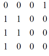
Fig. 3 below shows each element on the board and its neighbors considering a Moore neighborhood with periodic boundaries.
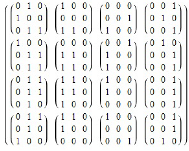
Fig.3 Moore neighborhood on initial grid
462
IJMMMAS 2017
It is possible to determine the number of living neighbors in each of the initial positions, counting the numbers of living neighbors which are around each cell:

Comparing the state of each cell of the game board in time tand the number of living neighbors, the following state in time t + 1 can be set up.
Fig. 4 below shows the transition from initial time t = 0 to t = 1. To visualize some examples, if we consider de state of de second element on first board row, it has 3 living neighbors so this cell will be born at t = 1 but first cell on third row of the board will be dead at next turn due to overpopulation.
463
IJMMMAS 2017
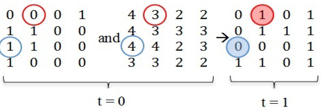
Fig.4 Evolution from t = 0 to t = 1.
Fig. 5 shows evolution from 1=t to 2=t. On the last row of the game board two cases of surviving rules are highlighted.
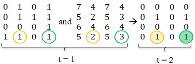
Fig.5 Evolution from t = 1 to t = 2.
464
IJMMMAS 2017
At the time instance t = 3, a board with all dead cells is obtained as shown in Fig. 6 below. The following turn, time t = 4, the same result will be obtained, so the game will finish by obtaining two consecutive similar states.
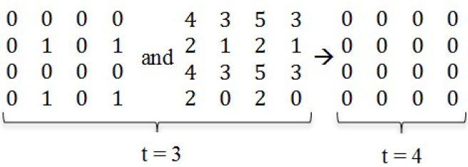
Fig.6 Evolution from t = 3 to t = 4.
4 LABORATORY PROJECT: DEFINING AND DEVELOPING A COMPUTATIONAL SIMULATION MODEL
In the context of meaningful learning, the students' activities must be oriented in a school system based on research and development of appropriate strategies for connecting and integrating the computational mathematics and the basic
465
IJMMMAS 2017
technologies and applied in Engineering to promote the multidisciplinary approach to the curriculum content corresponding to the plans of study, aiming to train professionals capable of solving complex models with the use of technologies.
The existence of simulation tools transformed the programming environments toward more collaborative spaces, with the updated listings of increasingly complex systems but with broad application in the various areas that comprise the engineering, it is possible to design methodological strategies that integrate the knowledge of the compartmentalized disciplines.
The developments that have experienced the mathematical software and the affinity that the students have to be linked with the technologies, imposes on the university teachers makes the effort to transform the teaching-learning process in the process of learning investigating [10].
The present experience shows the representation of the Game of Life using specific software (MATHEMATICA, Wolfram Research). To do this, the board and the way neighborhood for each cell is obtained as well as the transition rules should be set up.
The board is represented by a square matrix of order 4 St,
466
IJMMMAS 2017
and each of its entries is the state of a particular cell at a given time t.
The following step is to define the function which returns the number of neighbors alive of each cell of the board. To model this automaton, the Moore neighborhood is considered which is made up by the 8 neighbors around the position which is often identified with a cardinal point according to the position of the central cell: north, northeast, east, southeast, south, southwest, west and northwest. Fig. 7 below shows this Moore neighborhood.
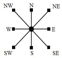
Fig.7 Moore neighborhood
It is possible to obtain a matrix that shows a particular neighbor by performing elementary operations on St.
467
IJMMMAS 2017
For example, to obtain a matrix Nt whose elements nij represent north neighbor of each site sij in St at a certain time t, it is necessary to move down every row on St by properly interchanging them. Ec. (1) shows N0that is north neighbors of each site ijs at time t = 0
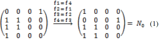
To find the matrix NE0 whose elements represent the neighbor in then Northeast position of each sij in S0 , first move the rows (f) downwards as shown in (1) above and then, on this resulting matrix, interchange columns (c) to the left. See (2) below.
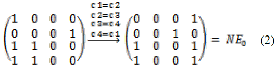
468
IJMMMAS 2017
Similarly, it is possible to obtain matrices that show a particular neighbor for each position in the state space and therefore to know the number of living neighbors of ijs adding these 8 matrices of neighbor positions.
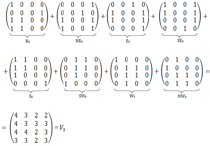
Fig.8 Number of living neighbors’ matrix at t = 0
469
IJMMMAS 2017
Fig. 8 above shows how to obtain number of living neighbors matrix at time t = 0.
Analyzing values of homologous elements on St and Vt , the next state into which sij will evolve can be obtained.
The evolution rule is function to the state of a cell sij and the number of living neighbor which it has.
Rule [stij : cell state sij ,vtij : number of living neighbors sij ] = st + + lij .
A living site with two living nearest neighbor sites remains alive: Rule[1,2] = 1.
Any site (no matter if living or dead) with three living nearest neighbor sites stays alive or is born: Rule[_,3] = 1.
All other cases, one cell either remains dead or die: Rule[_,_] = 0.
The following matrices: S0 ; S1 ; S2 ; S3 and S4 show the consecutive states which the game reaches at each instance t . Matrices can be represented graphically with a black site for living cells and a white one for dead cells. Fig. 9 shows both representations.
The number of different 2D geometric cellular automata that can be constructed from all possible rules is unimaginably
470
IJMMMAS 2017
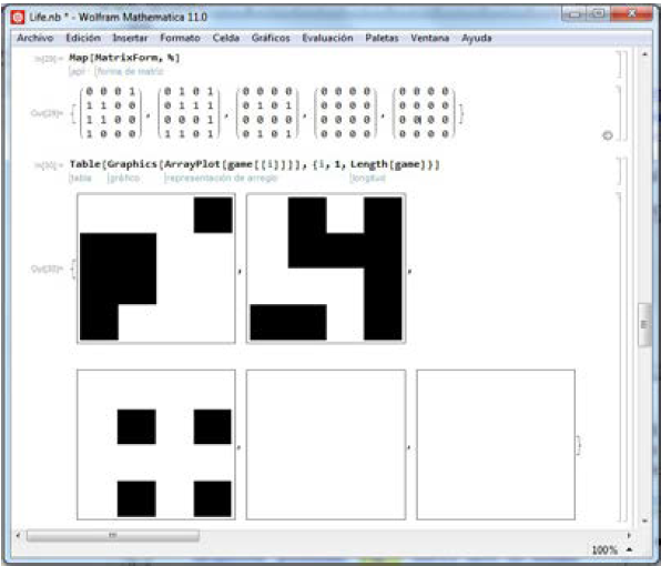
Fig.9 Game consecutive states
large. For simple binary cells, with 8 neighboring cells there are 8+1 cells that influence a given cell (previous state of a cell can influence it’s next state), which leads to 2512 possible binary
471
IJMMMAS 2017
combinations or approximately 10154 different CAs, of which the Game of Life is only one of them. In general, for an Nth Dimensional Geometric CA with (m) neighbors, there are 2k possible rules available for the Cellular Automata, where k = 2 m + 1 [11].
Game of Life rules are simple enough for anyone to understand, yet they lead to an endless number of different patterns, and to significant complexity [11]. Such as gliders, guns, puffers, ‘oscillating’ particles with different translation rates and spontaneous particle emission from some oscillating patterns among others.
It is interesting to observe different these patterns or life forms. In the evolution space there are four classes of behavior:
1) Evolution leads to a homogeneous state, in which all cells eventually attain the same value
2) Evolution leads to either to either simple stable states or periodic or separated structures
3) Evolution leads to chaotic nonperiodic patterns
4) Evolution leads to complex, localized propagating structures.
One of the most intriguing pattern is an oscillatory
472
IJMMMAS 2017
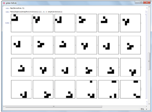
Fig.10 Glider pattern
propagating pattern known as glider, shown in Fig. 10, it consist of five living cells and reproduces itself in a diagonally displaced position once every four iteration.
Software allows visualizing an animation of any pattern evolution, shown in Fig 11. Glider gives the appearance of walking across the screen.
473
IJMMMAS 2017
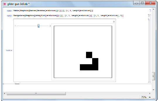
Fig.11 Glider pattern animation
There are some distinct moving self-replicating figures, which are individually referred to as spaceships. Unlike the glider, these spaceship figures are horizontally displaced. See Fig. 12
474
IJMMMAS 2017
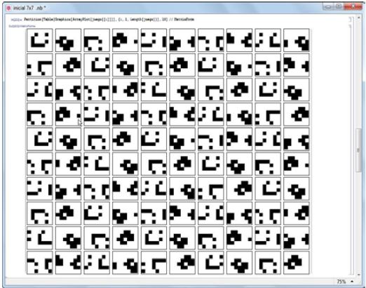
Fig.12 Spaceship pattern
475
IJMMMAS 2017
Fig.13 shows a pattern that disappears within a number of iteration:
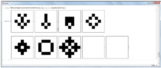
Fig.13 Cross pattern
Some initial configurations reach a stable state which does not change or disappear, as seen in Fig. 14.
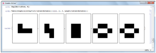
Fig.14 Stable pattern
476
IJMMMAS 2017
Live cells survive only if surrounded by two or three cells and a new cell is born only if surrounded by exactly three living cells. Initial configurations consisting of either single or neighboring live cells immediately yield the null state.
Survival in Game of Life requires a minimum of three living cells. Fig.15 shows the fate of one three-live initial state; its evolution is a period-2 state. Structures that lead into a periodic behavior are called oscillators.
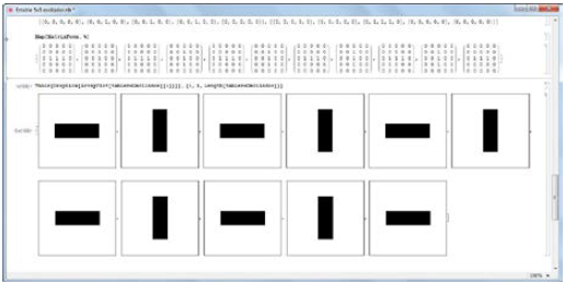
Fig.15 Oscillator
In general, it’s not possible to predict whether a particular starting configuration will eventually die out or not. There is no
477
IJMMMAS 2017
short-cut rout to the final outcome of this game’s evolution, it is necessary to await game’s own final outcome.
Combining several gliders in one single lattice produces different behaviors. Fig.16 below shows evolution resulting of combining two gliders placed in two opposite corners of a rectangular lattice. Game reaches null configuration in seventeen time-steps.
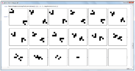
Fig.16 Evolution of two gliders
Fig. 17 below shows game’s evolution from a starting configuration that combine three gliders placed in different corners of a rectangular lattice. The final state of this pattern is a stable oscillatory pattern.
478
IJMMMAS 2017
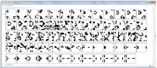
Fig.17 Evolution of three gliders
Placing four oscillator patterns on the same board evolves into a stable pattern after nine iterations as shown in Fig. 18 below.
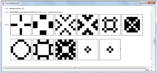
Fig.18 Evolution of four oscillator pattern
479
IJMMMAS 2017
From Fig. 19, we observe a pattern, called R-pentamino, which evolution is wildly unstable, expanding outward and continually undergoing change while scattering various bits of debris in all directions. This continues for many iterations steps marking a time beyond which all the various local patterns remain isolated and noninterracting. The significance of this evolution actually lies in the appearing of the oscillatory and propagating pattern known as glider [11].
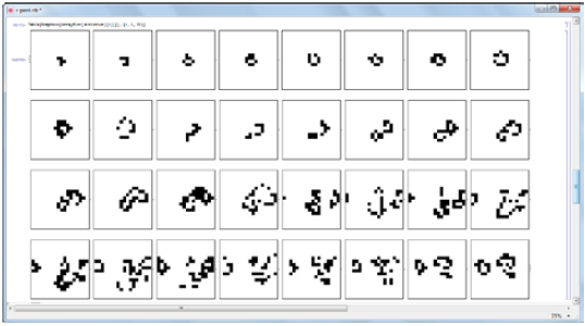
Fig.19 R-pentamino initial evolution
Students investigated these patterns and modified initial set-up
480
IJMMMAS 2017
to watch diverse evolution processes of the game. Laboratory work classes are an integral part of any educational program and their purpose is bringing the students closer to real situations of the area of studies.
5 ENGINEERING APPLICATION: POLLUTANT DIFFUSION IN A LIQUID FORM
CA application is the pollutant diffusion in a liquid form, for example the water flows which are presented in the projects of environmental remedial. In fact, this tool can be useful to guide and support the processes applied to purify contaminated water. It is not easy to obtain a numeric solution from a mathematical expression for such a phenomenon. However, there are ways to approach the problem by mathematical modeling of fluid transport: some of these methods will be studied in higher courses of engineering careers, CAs often provide a simpler tool that preserves the essence of the process by which complex natural patterns emerge [12].
481
IJMMMAS 2017
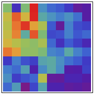
Fig.20 Initial concentrations of pollutant
Fig.20 shows a model of a liquid form with high pollutant concentrations on the high left corner of the analyzed section.
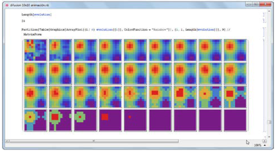
Fig.21 CA Simulated Pollutant Diffusion
482
IJMMMAS 2017
Fig. 21 above shows the evolution of the pollutant diffusion throughout time until all section under analysis is covered and a constant concentration is reached: Students are required to interpret the software graphic output of pollutant diffusion and to compare it with other software outputs which can result from changing the initial configurations of the pollutant concentrations. This mathematical model is applied to understand the distribution of pollutants by formulating a 2D diffusion.
6 CONCLUSION
The CAs have been used in different disciplines successfully. Currently, attention is raised towards the development of models which can carry out complex tasks such as cryptography, image processing and turbulence analysis, among others.
This is the reason why we consider important to introduce CA concepts and applications in engineering teaching, taking as a starting point the study of mathematical models with discrete variable systems.
483
IJMMMAS 2017
By introducing experiences as the ones described in the present paper for Algebra and Analytical Geometry, we search for a change of perspective which can see algorithms as a mathematical key activity and computer science as complementary knowledge to run those algorithms and manage their outputs.
Strategy design is highlighted as the outset of the study of mathematical models to solve discrete variable problems integrating the computational mathematics with the technological areas of the engineering curriculum while incorporating new learning styles.
REFERENCES
1. G. Merino, “Use of a Cellular Automaton to Create a Diffusion Model of Pollutants in a Soil-Water System”. Journal of Mathematics: Theory and Applications, vol.18, no.1, 2011, pp. 63-76.
2. A. Ilachinski, “Cellular Automata: A Discrete Universe”, World Scientific, 2001, pp. 175-185.
484
IJMMMAS 2017
3. J. Quartieri, N. Mastorakis, G. Iannone, C. Guarnacci, “A Cellular Automata Model for Fire Spreading Prediction”, Proceedings of 3rd WSEAS International Conference on Urban Planning and Transportation, 2010, pp. 173-179.
4. M. Dascalu, G. Stefan, A. Zafiu, A. Plavitu, “Applications of Multilevel Cellular Automata in Epidemiology”, Proceedings of the 13th WSEAS international conference on Automatic control, modelling & simulation, 2011, pp. 439-444.
5. R. Gaylor, P. Wellin, “Computer Simulations with Mathematica: explorations in complex physical and biological systems”. Springer-Verlag, 1995.
6. M. Resnick, “Turtles, Termites, and Traffic Jams”, MIT Press, 1994.
7. S. Wolfram, “Cellular automata as Model of Complexity. Nature, vol. 311, no. 5985, 1984, pp. 419- 424.
8. R. Gaylor, K. Nishidate, “Modeling Nature: Cellular Automata Simulations with Mathematica”, Springer-Verlag, 1996.
485
IJMMMAS 2017
9. J. Muñoz, “Autómatas Celulares y Física Digital”, Memorias del Primer Congreso Colombiano de Neuro Computación.
Academia Colombiana de Ciencias Exactas, Físicas y Naturales, Bogotá, 1996.
10. A. Tinnirello, E. Gago, M. Dádamo, M. Valentini, “Design, Simulation and Analysis of a Fluid Flow System through Multiphysics Platform”, Proceedings of 7th International Conference of Education, Research and Innovation, 2014, pp. 5847-5855.
11. T. Ostoma, M. Trushyk, “Cellular Automata: Theory and Physics. A New Paradigm for the Unification of Physics”, Cornell University Library, 1999.
12. S. Wolfram, “Computer Software in Science and Mathematics, Scientific American”, vol. 251, 1984, pp. 188-203.
486
INTED 2018
COMPUTATIONAL METHODS: THEIR ADVANTAGES ON TEACHING COMPLEX FLUID FLOW SYSTEMS Descargar pdf
A.M. Tinnirello, E.A. Gago, M.F. Romero
Universidad Tecnológica Nacional (ARGENTINA)
Abstract. The experience we communicate focuses on designing a class activity based on the integration of
content from various disciplines through an approach which supports mathematical models that
connect theoretical knowledge with real systems, thus making the applied equations, the interpretation
of the manipulated parameters and the results obtained meaningful. Using simulation software in
advanced Mathematics courses optimizes teaching-learning process since students can observe
phenomena and design the physical systems associated with specific applications.
Theoretical mathematical contents taught in an isolated and disconnected way do not facilitate the
students’ skills required to
487
INTED 2018
develop competence in higher levels of the career. As analytic methods are
not usually satisfactory to solve partial differential equations in certain boundary conditions, for nonideal
fluids, using computational methods becomes relevant to obtain solutions and analyze
behaviors.
We designed a laboratory experience to analyze the boundary layer flow between a viscous fluid and
a solid using the COMSOL Multi-physics simulation software in order to present partial differential
equations through the application of the finite element method. By means of numerical simulation and
basic knowledge on fluid flow, simple problems are introduced using a software platform both to
evaluate the importance of results obtained in an analytical and symbolic way, and to enhance
learning possibilities offered by virtual laboratory which supports disciplinary integration activities.
Keywords: simulation, computational mathematics, fluid flow, mathematical modelling.
488
INTED 2018
1 INTRODUCTION
The incorporation of technological resources in Higher Education allows to make substantial changes
in the programs of engineering careers, because they facilitate the understanding and integration of
the knowledge that students have in a compartmentalized way through the application of a tool that
favors training of the professional profile.
The development of numerical methods and the emergence of simulation platforms applied to
teaching, consider the need to guide the methodological approach of Mathematics programs towards
new forms of learning that impact a priori on the cognitive development of the student, and in the
future in a solid mental structure capable of solving problems of different kinds [1].
It is not about imparting knowledge using computer resources with abstract applications, which are not
useful, but to look for models applied to engineering that incentivize the implicit capacities that
students possess and that channel them to seek new ways of reasoning, fostering creativity and the
acquisition of critical and reflective thinking.
489
INTED 2018
The Multiphysics simulation software allows students to experiment in environments that approximate
reality, where the possibilities of learning significantly and with motivation increase exponentially. In
addition, it improves understanding and facilitates the learning of complex contents when trying to
learn processes of fluid circulation for educational purposes, processes that the student could not
observe and reason in the absence of these resources [2].
This work relates a multidisciplinary laboratory experience that was coordinated between different
chairs with the purpose of analyzing the Theory of the limit layer existing between a fluid that
circulates through a pipe when it encounters a spherical obstacle.
The platform COMSOL Multiphysics is used. It conforms a practical alternative for all kind of
experiments, because it allows to analyze the systems in different scenarios and geometries at low
cost, with no human risks and saving time and effort [3].
490
INTED 2018
2 METHODOLOGY
The applied methodology aims to create a learning space where a set of experimental activities are
developed as a fundamental line of the educational process. The programmed activities do not
separate theory of practice and are developed in the Basic Sciences Area Laboratory, where the
students perform technological applications with topics developed in class, linking the subjects of the
subject with different levels of the area, as well as with other disciplines Through the resolution of
models whose complexity is conditioned only by the basic knowledge that students have.
The teaching strategies are established from different practical activities without neglecting the
theoretical foundation, respecting the multidisciplinary approach [3].
In the areas of applied technology cycle and following a multidisciplinary line, training activities are
proposed, with a strong focus on professional activity. The design of the activities must present clear
objectives and goals that allow updating and continuously coordinating the tasks in the areas of
knowledge of university studies.
491
INTED 2018
It is essential that students, from the initiation to the completion of their studies in their chosen field,
use computational methods tending to represent the future work environment. This will strengthen the
unified vision of the student between Mathematics and its applications and will provide the essential
tools for their professional work.
The potential to profound and integrate the basic concepts, as well as to awaken the interest of
students in the incorporation of new topics, serve to incorporate concepts that can lead to a constant
search for new knowledge [4].
Integrating the knowledge acquired horizontally (subjects of the same year), and preparing students
for vertical integration (subjects of the upper cycle), that is, making the resolution of situations more
complex with the incorporation of new knowledge, different activities are designed.
3 OBJETIVES
• Use a Multiphysics simulation platform to analyze dynamic systems and compare of analytical
or numerical traditional calculation methods.
492
INTED 2018
• Value the benefits of plan different assumptions in a safe work environment, without any risk
and propose diverse alternatives, since multiple tests can be performed in a short period of
time.
• Analyze the pros of Creeping Flow de COMSOL Multiphysics modules, in the study of
program fluid fluxes in general, and the limit layer theory in particular. [4], [5].
• Evaluate the capacity that the program has when making changes in the parameters of the
system and its response.
• Evaluate the results obtained once the simulations have been carried out and arrive at
pertinent conclusions about the virtual system when applied in a real environment.
4 EXPERIENCE DEVELOPMENT
The Lab experience propose analyze the behavior of limit layer generated by the interaction of a fluid
in contact with a solid body.
With that purpose, commission groups of three participants each was created, and the session was
structured in the next way:
1- Search, analysis and selection of bibliography material.
493
INTED 2018
2- Case Analysis.
3- COMSOL Multiphysics software simulation.
4- Conclusions and analysis results.
Throughout the experience, we counted on the advice of the teachers in charge and they came to
address the theoretical concepts necessary for the work proposal. Then there was a debate on the
subject formulating the following theoretical framework:
In fluid mechanics, the limit layer or boundary layer is a manifestation in an area of the trajectory of
fluid movement that is disturbed by the appearance of a solid with which it comes into contact. The
boundary layer is explained as one in which the velocity of the fluid relative to the moving solid varies
from zero to ninety-nine percent of the velocity of the undisturbed current [5].
The region of flow above the plate and limited by the thickness δ (Fig. 1) is the boundary layer zone, in
which the effects of viscous shear forces caused by the viscosity of the liquid are felt, and it is almost
null by of the plate.
The boundary layer can cause laminar or turbulent flow; although areas of laminar flow and turbulent
flow can also
494
INTED 2018
coexist in it. Sometimes it is useful for the boundary layer to be turbulent [5], [6].
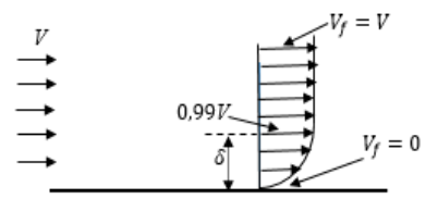
Fig.1 Fluid layers relative velocity
In aeronautics applied to commercial aviation, they usually opt for wing profiles that generate a
turbulent limit layer, since this remains adhered to the profile at greater angles of attack than the
laminar limit layer, thus preventing the profile from stalling. So, it stops to generate aerodynamic
sustentation in an abrupt way by the loss of limit layer [7].
The thickness of the limit layer in the area of the leading edge is small, but increases along the
surface. All these characteristics vary depending on the shape of the object (lower thickness of the
limit layer, the lower the aerodynamic drag present on the surface).
495
INTED 2018
Students analyze the effect of the limit layer by developing two models: the flow in the neighborhood of a flat sheet, and the flow around a sphere, to perform this task work through the following stages: Design of work geometry, Mesh and System modeling.
4.1 Geometry Design
In first stance, Work geometry is defined with the purpose of modeling the systems and define their restrictions. The platform allows generate 2D and 3D geometries, having the schemes that are shown in Fig 2 and Fig 3.
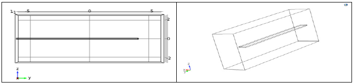
Fig.2 2D and 3D fluid-thin plate geometry system.
496
INTED 2018
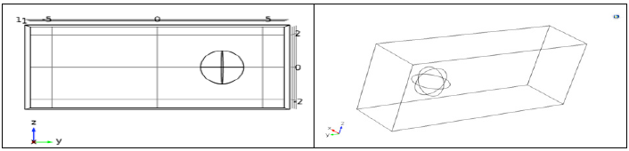
Fig.3 2D and 3D fluid-sphere geometry system.
In both cases, the fluid is water. Both the thin plate and the sphere are made of iron. The Software has
incorporated a list of material that considers their physical properties, and in this study the students
decided to work a constant temperature.
In those graphics are observed the contour conditions imposed for the fluid-thin plate and fluid-sphere.
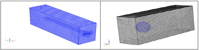
Fig.4 Meshing geometry.
497
INTED 2018
4.3 Modelling System
In the study of fluid flow, it is important to consider hypotheses about variations in density versus
changes in pressure and temperature. The application module of the software is intended for fluids
that are incompressible, however, small changes in density are allowed [5], [8].
The equations with which COMSOL works are those of Navier-Stokes and describe the physical
parameters that sometimes determine the coupling of several physics, this turns out to be a primordial
quality granted by the technology that is applied.
Each of the physical which includes the program, are bounded by a system of equations that allow you
to perform the analysis in the model. You can also modify the equations which are defined in the
program, either manually or with the help of a specific module [5].
The analysis of the relationship of the mechanisms of transport is achieved from a system of
equations formed by the Navier-Stokes equations and the continuity equation for isothermal flow not
steady-state.
498
INTED 2018
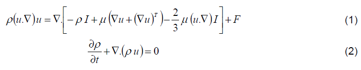
Where: ρ : Density, u : Velocity flow. μ : Dynamic viscosity. I : Identity matrix. T : Temperature.
F : Constant.
In addition, the Navier Stokes equation takes into account the density constant in the term convective
and discarded the effects of the turmoil.
5 RESULTS
5.1 Fluid-plate System
Tests are carried out considering that the fluid circulates at velocities of 0,01 m/sec and 0,10 m/sec
whose effects are observed in Fig. 5 and 6, respectively.
The students analyze the graphs provided by the software and note that the flow stream lines in the
boundary layer are approximately parallel to the plate and to the fluid flow current.
499
INTED 2018
At points close to the surface of the plate the velocity tends to be zero. In the neighborhood of the
stela surrounding the solid, there is a relatively small area where the velocity of the fluid is
approximately the same as it was when it circulated before encountering the plate, and after that area,
and by effects of the boundary layer the velocity increases considerably, but the pressure gradient is
constant and of very small magnitude through the boundary layer.
When the fluid current moves away from the plate, the velocity of the plate slowly stabilizes until after
a short time it returns to its original value.
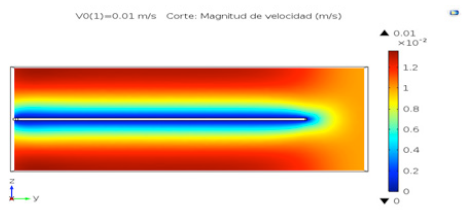
Fig.5 Fluid velocity variations.
500
INTED 2018
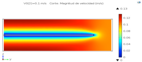
Fig.6 Fluid velocity variations.
When the students analyze the pressure gradients, they observe that fluid possess a high pressure in
the instant at the point of stagnation after the plate, despite this pressure gradient, the fluid does not
change its velocity after leaving the plate [9].
The pressure decreases after it moves away from the plate, where the fluid force is not capable to
surpass the forces by the internal friction, so this produces pressure gradients in opposite directions.
As velocity is increases, the pressure effect at stagnation point increases significantly.
The systems pressure gradients for velocities of 0,01 m/sec and 0,10 m/sec are observed in Fig. 7
and 8, respectively.
501
INTED 2018
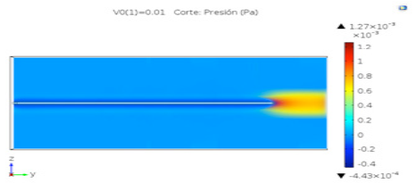
Fig.7 Pressure gradients.
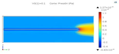
Fig.8 Pressure gradients.
5.2 Fluid-sphere system
A parametric sweep is made for different fluid velocities, in order to observe the behavior of the limit layer that forms around the
502
INTED 2018
solid material and the variations in velocity and pressure that the fluid
presents.
Tests are carried out considering that the fluid circulates with velocities of 0,01 m/sec and 0,10 m/sec
and whose effects are seen in Fig. 9 and 10, respectively.
In Fig. 9 and 10, students observe that the flow has the characteristics of boundary layer, where the
velocity profiles of the fluid that circulates from left to right are considered with a plane of cut located in
the center of symmetry of the sphere.
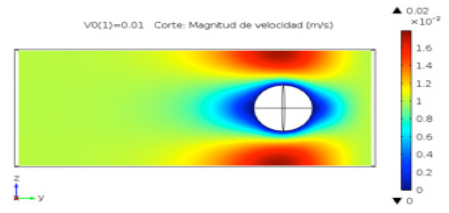
Fig.9 Fluid velocity variant.
503
INTED 2018
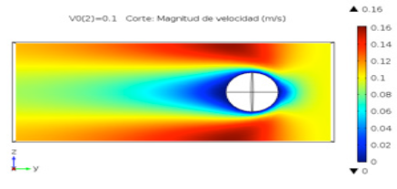
Fig.10 Fluid velocity variant.
At points close to the surface of the sphere the velocity tends to be zero. In the vicinity of the wake
that surrounds the solid, there is a relatively small area where the velocity of the fluid is approximately
the same as it was when it was circulating before hitting the sphere, and then from that zone and by
effects of the boundary layer the velocity It grows considerably since the pressure gradient is favorable
(the area that is distinguished with red color in the graph) [10].
It is also observed that the fluid moves away from the sphere, forming vortices and instability of the
fluid, to then stabilize the velocity of this.
With the intention of seeing how the wake would be observed
504
INTED 2018
around the sphere when the velocity of the fluid circulation increases considerably, we work with a velocity of 5m/sec and as seen in Fig. 11, it is seen that the blue wake it widens to the left around the sphere.
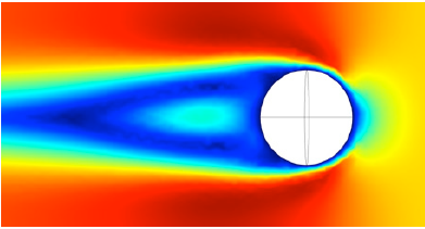
Fig.11 Fluid velocity variant.
Through the graphical interface of the software, different cuts can be made through different planes of
the geometry observing the flow patterns in the different model sections.
For greater visibility, the example is shown in Fig. 12 for a velocity of 5 m/sec.
505
INTED 2018
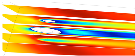
Fig.12 Fluid velocity level surfaces.
The pressure is another parameter that can be analyzed in this type of phenomena. In Fig. 13 and 14
it is observed that, unlike velocity, the fluid pressure increases to the right of the sphere.
The flow impinges on the sphere, causing a high pressure at the point of later stagnation. Due to this
pressure gradient, the fluid accelerates as it travels around the contour of the sphere, and the
pressure decreases after it moves away from the sphere, where the force of the fluid is not able to
overcome the viscosity of the sphere what will eventually form pressure gradients in the opposite
direction. The analysis for the fluid pressure gradients is carried out for velocities of 0,01 m/sec and
0,10 m/sec.
506
INTED 2018
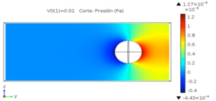
Fig.13 Pressure gradients.
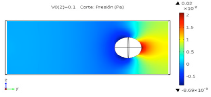
Fig.14 Pressure gradients.
In Fig. 15 and Fig. 16, the level curves corresponding to the pressure gradients in 2D and 3D are observed for the velocity 0,01m/sec.
507
INTED 2018
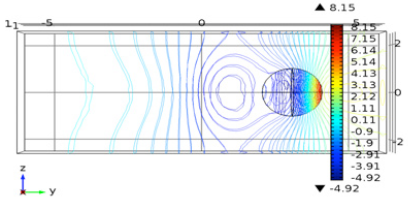
Fig.15 2D pressure levels curves.
The fluid impinges on the body and tends to follow its contour. After crossing it, at the back of the sphere in the direction of the fluid path, you can see how the closest flow lines follow the movement of the vortices that are created, the furthest away from the solid, they do not show any kind of disturbance but as the lines approach the sphere they present small oscillations.
507
INTED 2018
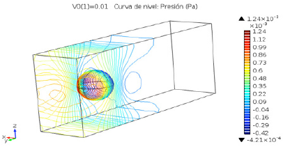
Fig.16 3D pressure levels curves.
6 CONCLUSIONS
The purpose of incorporating Multiphysics simulation platforms in university education is to establish a
nexus between basic sciences and applied technologies, since they produce changes in the different
learning structures, promoting the development of students' abilities.
In the experience it is shown, relating to previous works, how the same situation that can be analyzed
with the complex variable, in the case of the boundary layer, is insufficient for its resolution, and the
simulation software provides a real response to the model.
509
INTED 2018
The activity developed encourages students to carry out a self-managed work, and they gain
independence by acquiring skills to work in problematic situations. By means of numerical simulation
and basic knowledge of fluid flow, simple problems are introduced using an environment such as that
offered by the COMSOL platform to evaluate the importance of the results obtained in an analytical
and symbolic way, and to enhance the learning possibilities offered by the use of the virtual laboratory
to support disciplinary integration activities.
The study of the flow around a sphere is done in the university field most of the time in an
experimental way, performing laboratory practices, without incorporating the benefits of having a
laboratory with adequate technology. In addition, the advantages of the use of simulation technology
are demonstrated by the visualization of the high velocity and temperature gradients that occur in the
flow around the sphere, as well as by the non-permanent nature of the resulting flows.
510
INTED 2018
REFERENCES
1. K. Sumithra, A. Dharani, M. Vijayalakshmi, “Transformation in Engineering Education: An
Analysis of Challenges and Learning Outcomes”, en Proc. of the 14th International Conference
on Education and Educational Technology, pp. 33-36, 2015.
2. A. Tinnirello, E. Gago, L. D’Alessandro, M. Dádamo, “Virtual Instruments Integrating
Mathematical Modeling for Engineering Education”, en Proc. of 9th annual International
Conference of Education, Research and Innovation, vol. 1, pp. 255-264, 2016.
3. A. Tinnirello, E. Gago, M. Valentini, Design and Simulation of Mechanical Equipment by Design
Tools and Multiphysics Platforms, Proceedings of 8th. International Conference of Education,
Research and Innovation, pp. 789-797, 2015.
4. R. Torres, J. Grau, Introducción a la mecánica de fluidos y transferencia del calor con Comsol
Multiphysics, España: Editorial Addlink Media, 2007.
5. R. Bird, W. Stewart, E. Lightfoot, Transport Phenomena, USA,
511
INTED 2018
Publisher: John Wiley, pp. 133-
144, 2006.
6. G. Bognár, and Z. Csáti, Numerical Solution to Boundary Layer Problems over Moving Flat
Plate in Non-Newtonian Media. Journal of Applied Mathematics and Physics, vol. 2, pp. 8-13,
2014.
7. J. Nagler, Laminar boundary layer model for power-law fluids with nonlinear viscosity, en
Proceedings of WSEAS Transactions on Fluid Mechanics, vol. 9, 2014.
8. J. Cengel, J. Cimbala, Mecánica de Fluidos: Fundamentos y aplicaciones, México: Editorial
McGraw-Hill, 2006.
9. F. White, Mecánica de fluidos, España: Editorial McGraw-Hill, 2008.
10. S. Admad, N. Md Arifin, R. Nazar, I. Pop, Mathematical Modeling of Boundary Layer Flow over
a Moving Thin Needle with Variable Heat Flux, en Proceedings of 12th. International Conference
on Applied Mathematics, pp. 48-53, 2007.
512
INTED 2018
ALGORITHMIC MATHEMATICS IN LINEAR ALGEBRA APPLICATIONS Descargar pdf
A.M. Tinnirello, E.A. Gago, P.A. Szekieta
Universidad Tecnológica Nacional (ARGENTINA)
Abstract. The aim of this paper is to provide a computational approach to Linear Algebra (AL) in order to tackle
the conceptual difficulties that this field of mathematics presents to students. Also, AL is considered
difficult in the curricula due to the high level of abstraction of the concepts involved. In the first-year
courses of Mathematics there are different issues which hinder the teaching-learning process, being
the most notorious the lack of basic knowledge which students who start university have. Therefore it
is essential to present simple models which can encourage students to develop new ways of thinking
and reasoning while triggering motivating teaching situations.
This experience is introduced in Algebra and Analytical Geometry subject with the purpose of
integrating linear transformation
513
INTED 2018
concepts and the use of mathematical software tools. The activities
presented aim at developing algorithms procedures so as to relate theoretical knowledge with
interesting engineering applications.
The methodology adopted to carry out the experience was carried out through theoretical lessons with
technology practice, where the contents of the linear algebra were given to develop simple geometric
models that would lead to a meaningful conceptualization of the topic. Students conducted an
exploratory activity by using and matching the theoretical concepts; from related transformations
different models, curves and surfaces were developed in 2D and 3D, looking for patterns of behavior
and their relationship with various applications. To address the methodological innovations described
above, curriculum adaptation to fit the generation of new learning systems cannot be postponed.
Keywords: simulation, lineal transformation, modeling, applications.
514
INTED 2018
1 INTRODUCTION
At the first year AL course, the issues that obstacles the learning process are diverse. Between them,
the inadequate basic formation with the students enters the university, so that makes essential to plan
simple models that leads to the acquisition ways of thinking and reasoning, and being triggers of
motivating situations.
This paper describes an experience in a course in Algebra and Analytical Geometry, in the Chemical
Engineering career, where students are expected to integrate knowledge when developing the topic
Linear transformations through the use of specific software. Situations are proposed by means of
which an analytical procedure is induced to relate the theoretical concepts learned in the classroom
and to enhance the competences that students can develop.
The vision of teaching Mathematics in engineering careers in Higher Education institutions, aims that
learning is done under certain conditions, which allow students to acquire knowledge with techniques
that are inherent to problems related to their future professional work [1].
515
INTED 2018
A central topic has acquired relevance, especially in engineering courses; The incorporation of
communication and information technologies in the educational field. It is fundamental that education
includes an applied work line to the digital technologies in their specific areas [2], [3].
To build the cognitive and attitudinal bases of a professional, it is necessary to encourage dedication
to research from the first level of the career. Particularly in the use of computer applications is
necessary to guide the student to track the baggage of knowledge that has in the use of computer
resources to the use of learning the concepts of Mathematics.
To address the methodological changes taking into account the above considerations, it is necessary
for universities to adapt to the progress and the generation of new knowledge through new proposals
in the activities developed in class.
2 METHODOLOGY
The Information and Multidisciplinary of Basic Sciences Laboratory is the physical space where a collaborative work environment is created. For this purpose, a workshop class is
516
INTED 2018
designed, which is
called the theoretical-practical-technological class where the concepts of the geometry of linear
transformations are applied in the plane and in the space, trying to introduce models that have an
entity in the field of Engineering and that in addition, they are related to the generation of objects of a
current mathematics [4].
The Laboratory class aims to train the student in specific software, with the intention that from the use
of computer resources can develop their inventiveness and dexterity, and conceptualize the content.
The characteristics of the theoretical-practical technological class are to establish the guidelines of an
interactive work of engineering analysis that manifests itself in an activity that produces new ideas.
This methodology of teaching and learning allows us to advance first with the theoretical research of
the subject, creating an environment where the student assumes an active role, leaving aside the fact
of being a spectator, and allowing him to build concepts through experimentation, and the elaboration
of conclusions.
The teacher, in this kind of experience, take the roll of process guide and acts like a facilitator of
learning, until reaching the full
517
INTED 2018
understanding of the subject under study, including with questions that activate a mechanism of continuity in the extension and subsequent investigation of different lines on the proposed problem.
3 OBJETIVES
The need to look for an alternative form of teaching that not only addresses the requirements of the
program, but motivates the students with the incorporation of application problems that are related to
the theory of the developed topic. Due to the low level of prior knowledge that students have in the first
year of engineering careers, it is known that in the area of AL it is difficult to find models that can be
understood by students, but it is necessary for teachers to try to look for problematic situations. that
awaken curiosity and motivation in students [5].
This restriction is also conditioned by the obstacles generated by the concept of Lineal Transformation
when it is presented to the student in the first instance.
In this experience it is proposed the use of a valuable tool: the symbolic calculus. It is used like a
connector of applied
518
INTED 2018
mathematical functions in real situations, which allows to validate the student’s
own skills for the basic competences development.
The interconnection between the concepts of LA, the real cases in the engineering field, and the
anticipation of knowledge that will later become more complex in the subjects that deal with basic and
applied technologies provide students with versatility when considering models each more
sophisticated times in the specific subjects of his career [5], [6].
It is about creating a work environment where the student can be reflective, critical, make decisions
and also define the mistakes made in the process. This situation incites the need for the student to
know the object of study and create the internal conditions for the assimilation, in an active and
independent way of the new knowledge.
4 EXPERIENCE DEVELOPMENT
A theoretical-practical-technological class is designed in two sessions of three hours chair each, in which students are to be led in a significant process of learning the proposed subject,
519
INTED 2018
through the
analysis of linear transformations and the relationship established with the geometric visualizations.
The stages designed to carry out the class are: assembly of the work groups, posing of a problematic
situation, revision and later selection of the bibliographic material on the subject, review of the
contents developed in the theory class, modeling of the situation, and resolution of the proposed
models and conclusions.
In the Laboratory class, we work with groups of students that do not exceed the three members, and
to achieve the expected task is presented cases of simple engineering applications and fractal
geometry, with the purpose that students rely on the use of computer tools.
The students have the freedom to form the groups according to their criteria and choose which group
they want to participate in, but it is set as an indispensable condition for working as a team, fostering a
collaborative environment. Each group has at least one desktop computer, but it is also allowed to
bring their personal computers to work.
In the first part of this experience, simple models related to the engineering work are presented and in
the second part of the
520
INTED 2018
class the generation of fractals is made from related transformations, which involve the concepts of linear transformations.
4.1 First session: Engineering application
4.1.1 Case 1: Center of gravity and transversal sector of a pipe.
A pipe has a transversal rectangular section as indicates on Fig. 1, and it is hanged from the ceiling in oblique position according an α angle with respect to the perpendicular that forms the ceiling with the wall. With the objective to analyze the air flux that will pass in the said enclosure, it is asked to the students to modify the pipe position and the transversal section, in a way that increases the amount of flux pass, and the center of gravity is positioned in the origin of coordinates.
521
INTED 2018

Fig.1 Pipe scheme.
In Fig. 2, shows a rectangle which represents the transversal pipe section, whose vertex are the coordinates points: A( − 5,657; 2,828); B( − 4,49; 3,995); C( − 0,424; − 0,071) and D( −1,591; 1,237).
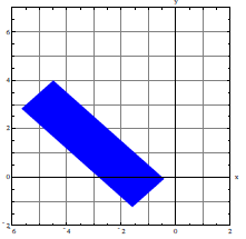
Fig.2 Oblique position pipe.
522
INTED 2018
According to the request, and after investigating the theoretical knowledge of the subject, the students suggest to use first the transformation of rotation expressed through Eq. (1), which allows to rotate the position of the pipe in order to keep the sides of it parallel to the ceiling, walls and floor.
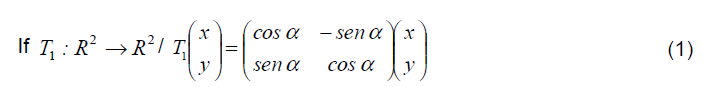
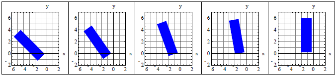
Fig.3 Pipe Rotation Sequence.
The students realize tests to determine the α angle value which places the pipe in the desired position, after try with various rotation angles, they find when α = 45º the vertical pipe position is achieved. Fig. 3 shows a sequence of some tests realized from the students until find the desired position [7].
523
INTED 2018
After Then, they select the mapping whose matrix transformation corresponds with the eq.(2), which produces a translation in the last graphic position of Fig.3, and places to the same origin coordinate center, as observed in Fig. 4.
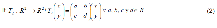
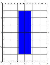
Fig.4 Pipe with its center of gravity on origin of coordinates.
Finally, to increase the pipe transversal section and allow to pass double amount of air, the students proposes the use of the Transformation stablished on the eq(3), which achieve not only keep the center of gravity, but also modifies its air pass capacity
524
INTED 2018
to double [8].

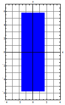
Fig.5 Double-sized pipe.
Consequently, it is indicated that if you know the cross sections of two pipes, one hexagonal and another square, located in different regions of the plane, you are asked to analyze which linear transformations you can propose to reduce them cross-sectional area and its center of gravity is the origin of coordinates. The sequence in graphic form of the results obtained by the students is shown in Fig. 6 and 7.
525
INTED 2018
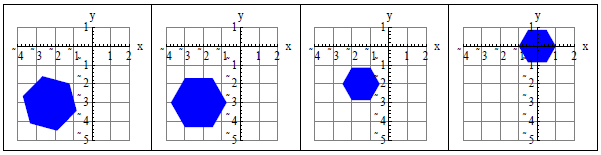
Fig.6 Transformations for a transversal section hexagonal pipe.
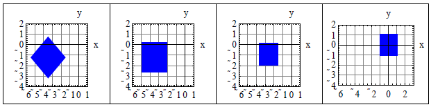
Fig.7 Transformations for a transversal section squared pipe.
4.1.2 Case 2: Fan Blades Design
In the design of pieces, it is advisable to start from a simple scheme, in order to study their properties and then make the corresponding transformations to obtain the desired shape. In general, the pieces that form the ventilation devices usually present symmetry with respect to the axis of rotation. It is then proposed to design the shape of the propellers of a fan. The
526
INTED 2018
students propose a simple graphing geometry that represents one of the blades of a fan as shown in Fig. 8 [9].
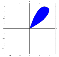
Fig.8 Fan Blade.
The students apply the transformation whose produces reflections respect to the coordinate axis. The eqs. (4), (5) y (6) corresponds to the reflection respect from y axis, reflection to x axis, and reflection in 3rd quadrant, respectively [7], [8].
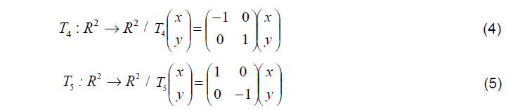
527
INTED 2018

The application of the transformations enunciated in (4), (5) and (6), is translated in the graphs of Fig. 9, where the transformations in the plane generated from the vane of Fig.8.
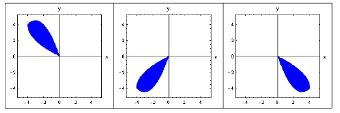
Fig.9 Fan Blades obtained by reflection of a Master Fan Blade.
The combination of the vanes of Fig. 8 and 9, allow to design the complete structure that have the blades of a fan. In Fig. 10 the combined arrangement of the fan blades designed from the application of the linear transformations is presented.
528
INTED 2018
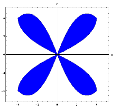
Fig.10 Fan Blades.
4.2 Second Session: Fractals Objects Generation
In principle, it is intended that students generate the fractal object called Sierpinski Triangle (ST),
analyzing the related transformations that will be used for this process. In this context, they begin the
experience starting from an isosceles triangle of vertex, and, and through the application of a system
of iterated functions (SFI) they will generate the desired geometric structure [10].
The laws of related transformations applied are:
529
INTED 2018
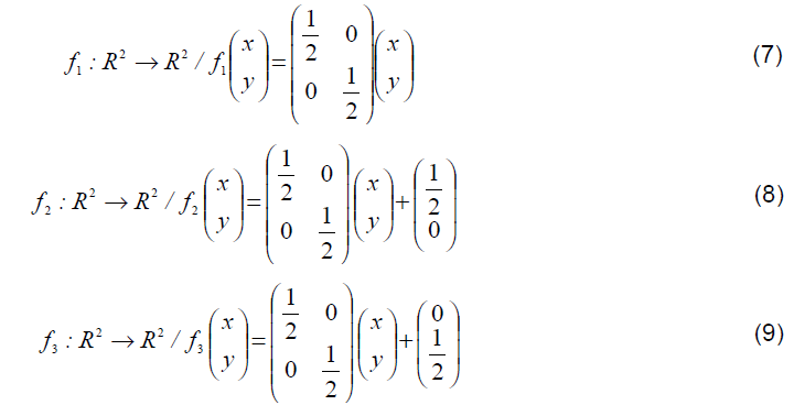
When they realize the first iteration on  applying the SFI, the generator whose is a divided triangle in four smaller triangles, is obtained [10].
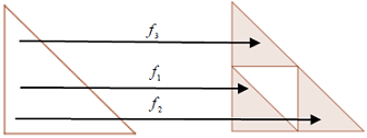
Fig.11 SFI application.
530
INTED 2018
From that point, and as consequence to keep applying SFI, the students achieve the first five graphics, observed in Fig. 12.
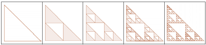
Fig.12 First ST iterations.
The iteration tending to infinity applying the SIF allows the students to generate the fractal called ST, in Fig. 13 the result of the experience is shown.
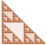
Fig.13 Finite ST representation.
As a result of this activity, and through the application of a new
531
INTED 2018
SFI, students will build a new entity called Sierpinski rug (AR), which according to the inquiry made in the investigation of the task requested, is a generalization of Cantor's set. To realize this compact object, the equations that respond to the model are [7], [10]:
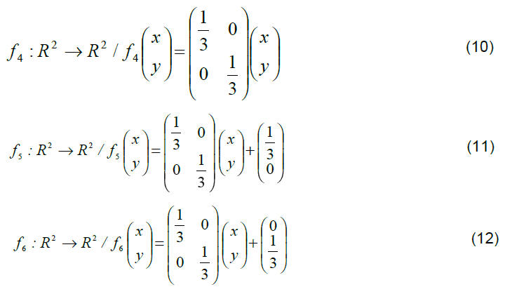
The graphs that they obtained regarding the construction of the AR are showed in Fig. 14 and 15.
532
INTED 2018

Fig.14 First application of SFI to the AR.
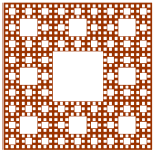
Fig.15 Generation of AR.
After generate the ST and the AR, the students analyzes similar structures but in space. The applied SFI in this case is {f7 , f8 }[8].
533
INTED 2018
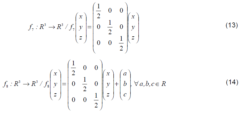
Starting from a tetrahedron and a cube, students are asked to begin with the process of forming a fractal object in R3 . In Fig. 16 and 17, the first 3D graphics obtained after applying the related transformations of the SFI are shown
534
INTED 2018
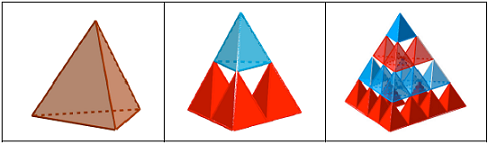
Fig.16 3D fractal from a tetrahedron.
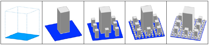
Fig.17 3D Fractal from a cube.
5 CONCLUSIONS
The use of linear transformations applied to the study of idealized models applied to engineering, along with the generation of fractal objects and the support of computer resources used appropriately led to a contextualized analysis that achieved the objective of understanding the subject,
535
INTED 2018
visualizing
the properties of reflection, rotation and translation that present the treated surfaces.
The relationships that the students could establish through visualization allowed them to conceptualize
in a fast and efficient way the topic of the mappings with the use of the matrices of linear
transformation, in addition not only new knowledge was incorporated but students continuously had to
appeal to review and investigate concepts related to the subject (product of matrices, the vision of
what linear transformation means as a function and alternatively how a matrix product, etc.)
After finishing the class, a synthetic evaluation was carried out that showed that the pedagogical
proposal made through this pilot test had a positive impact on the learning of the subject. In addition,
the students recognized the importance and the advantage of using specific software to generate the
fractals, and showed that this activity could be done because in our faculty we have a multidisciplinary
laboratory equipped properly.
In the future, we intend to develop other subjects of the subject in the Laboratory, and extend the
experience to courses of other engineering specialties within our Faculty with the aim of
536
INTED 2018
generating
basic skills in the area of Mathematics.
This experience is a link between the disciplines of the University Basic Cycle with the subjects of
basic and applied technologies, and allows to provide students with an autonomous character to
perform the required tasks and learn new knowledge, as well as creating a host of activities to address
problematic situations related to engineering tasks.
REFERENCES
1. R. Posada Álvarez, “Formación Superior Basada en Competencias, Interdisciplinariedad y
Trabajo Autónomo del Estudiante”, Revista Iberoamericana de Educación, 2011.
2. G. Bischof, E. Bratschitsch, A. Casey, D. Rubesa, “Facilitating Engineering Mathematics
Education by Multidisciplinary Projects”, Journal of American Society for Engineering Education,
2007.
3. M. Rosen, “Engineering Education: Future Trends and Advances”, Proceedings of the 6th.
WSEAS International Conference on Engineering Education, pp.44-52, 2009.
537
INTED 2018
4. S. Raichman, G. Sabulsky, E. Totter, E. (Coords), M. Orta, P. Verdejo, “Estrategias para el
desarrollo de innovaciones educativas basadas en la utilización de Tecnologías de la
Información y Comunicación”. En: “Estrategias para el uso de tecnologías de información y
comunicación en los procesos de aprendizaje”, Publisher Innova Cesal, México, pp. 19-34,
2013.
5. R. Posada , “Formación Superior Basada en Competencias, Interdisciplinariedad y
Trabajo Autónomo del Estudiante”, Revista Iberoamericana de Educación, 2011.
6. V. Macchiarola, “Currículum basado en competencias. sentidos y críticas”, Revista Argentina de
Enseñanza de la Ingeniería, Vol. 8,Issue 14, pp. 39-46,2007.
7. G. Nakos, D. Joyner. “Álgebra lineal con aplicaciones”, México, Publisher International
Thomson, pp. 365-369, 1999.
8. B. Kolman, D. Hill, “Álgebra lineal con aplicaciones y MATLAB”. México, Publisher Pearson
Addison-Wesley, pp. 520-536, 2006.
9. E. Carnicer Royo, “Ventilación industrial: Cálculo y aplicaciones”,
538
INTED 2018
Madrid, Publisher Thomson,
2001.
10. Z. Zhu, E. Dong, “Simulation of Sierpinski-type fractals and their geometric constructions in
Matlab environment” .Proceedings of WSEAS Transactions on Mathematics, 2013.
539